Workflow to determine Impington Mill's biotope using CFD
Workflow to determine Impington Mill's
biotope by Victor Reijs
is licensed under CC
BY-NC-SA 4.0


Introduction
On this webpage the wind biotope of Impington Mill is being evaluated.
First the making of the
CAD-model is described and after that the results
of simulations with a CFD.
At the end an
evaluation is given.
Several questions are outstanding, see
below purple text. If you have input, please let me know.
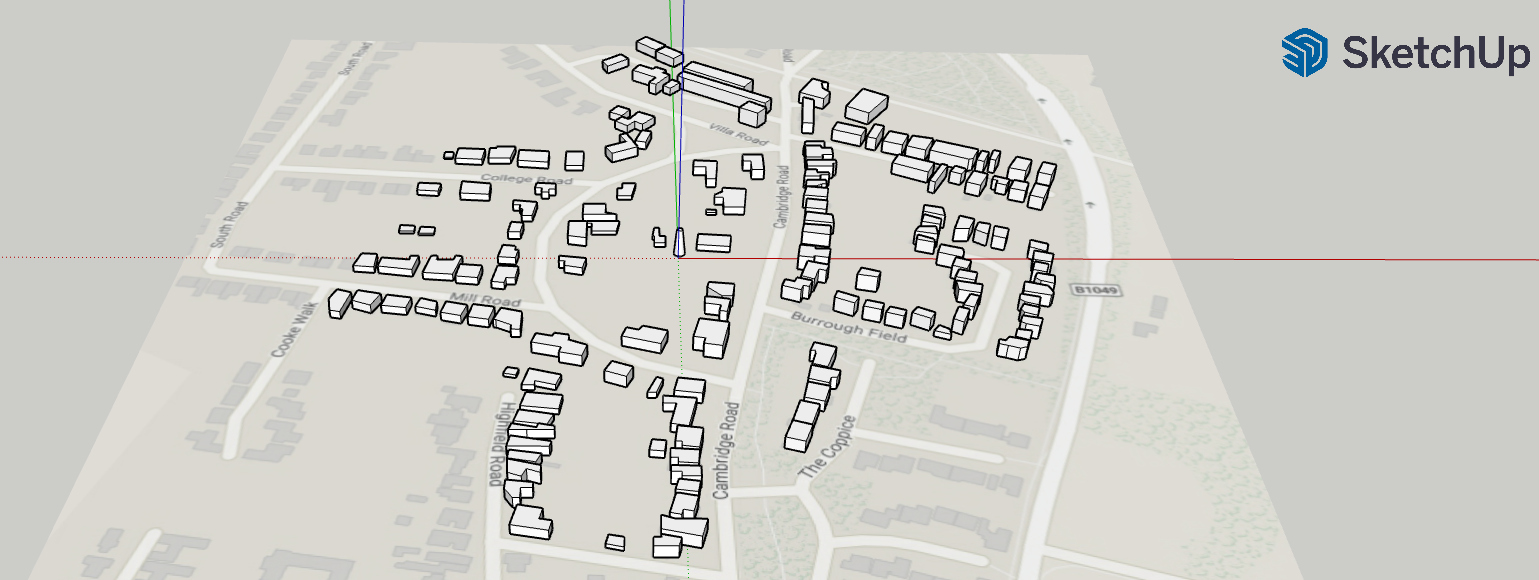
Making a CAD-model with SketchUp
SketchUp CAD-program is used to make
the CAD-model. SketchUp Free version
is well equipped for the windmill environment. In this program one
can easily make 3D forms, such as: boxes, roofed boxes, cylinders,
capped cones, trees, etc, etc.
Buildings that are around a windmill, say with a radius of 250m,
can be simulated by a box (with its height: the wall height plus
half the roof height); or otherwise a more precise model (box with
hipped roof, etc.). A windmill can be a simple standing
cylinder/capped cone. Don't go into too much details as that will
not have much influence on the CFD results.
Furthermore, buildings below the ground/bailey height are
certainly not in need of precise dimensions. As a guideline
include anything that is higher than the DHM-rule
minus 2m.
The following steps for making the CAD-model can be seen as a
guide line:
- Define in SketchUp the unit of the dimensions (CFD uses
m[etres], so do the same in SketchUp): Model Info (i) →
Length Units → Meter; Model Info (i) →
Display precision → 0.00 m; and Model Info (i)
→ Length Snapping → OFF
- One can add a piece map (500 by 500m with the mill in the
middle) from of Google Map (so when get an idea where buildings
are), use: ≡ → Add Location → Select Region →
Import
- Having imported this, one can now trace the contours of the
building-plans (Line-tool). Make sure you have zoomed in enough
as that is easier to trace. Make also sure that your buildings
all go down to a height of 0m. One can also disable Linear
inferences (OFF by using the Alt-button).
There is no real need to be very accurate (say within 0.25m).
- After tracing the contours of the building plans, one can
increase their height by extruding them (Push-Pull tool). At the
right bottom of the window (Measurements) one can see the
pull height.
- For UK there is the Defra Data Service which provides a
DSM (Digital Surface Model) for 2019 and 2022 (which uses British National Grid
and see also OS Maps).
- The GeoTIFF (DSM) file has been changed into a csv file by
using a small program in R. This csv file has been imported in
Excel for presentation and easy viewing.
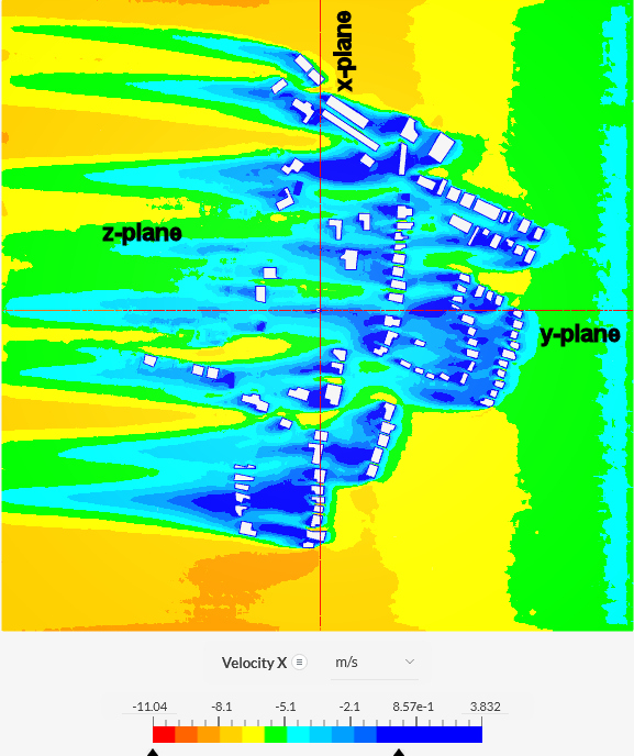
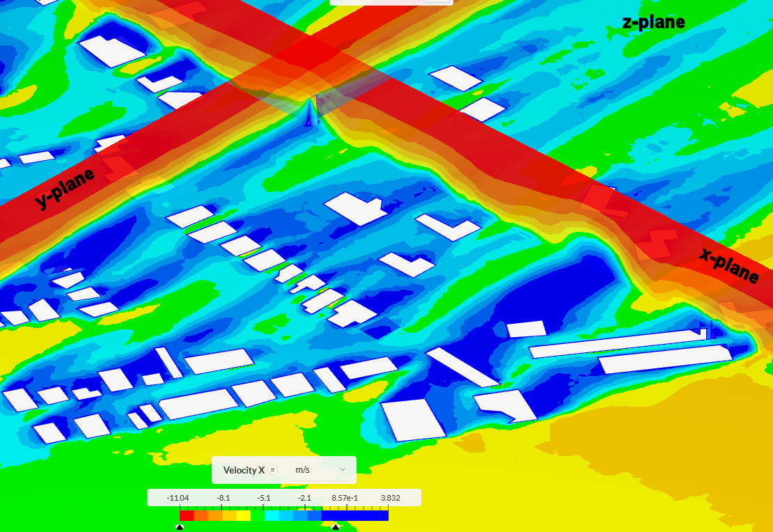
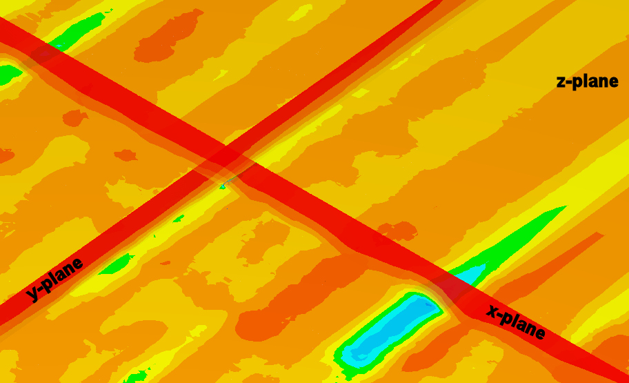
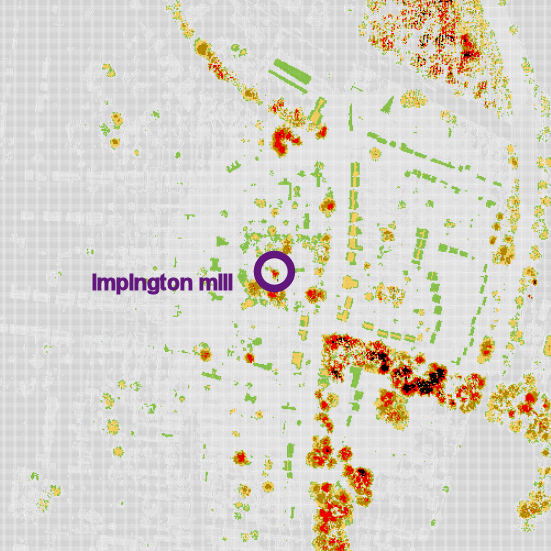
- Here is the 2022 DSM (Digital Surface Model: green lowest;
red highest) for an area of 500*500m with Impington Mill in
the middle (top is North; bottom is South; right is East; and
left is West):
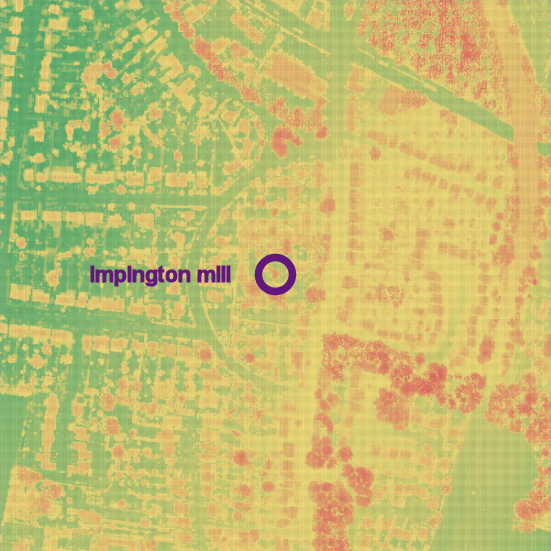
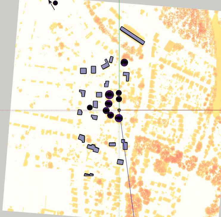
- Using the DHM-rule
on this 2022 DSM, one gets the following picture (top is
North; bottom is South; right is East; and left is West):
The colouring gives a height referenced
from the DHM-rule: green from -2 to 0m; orange from 0 to
4m; brown from 4 to 8m; red from 8 to 12m; black: above
12m
- For simplicity one simple use a box for a roofed
building: with its height: height of walls + half of height of
roof.
There is no real need to be very accurate (say within 0.25m).
See for a further study here.
- The mill is made by using a circle (Circle-tool), pull up
(Pull tool) to form a cylinder (or capped cone): height of cap
is 16.2m, and windshaft height is around 15m.
- Make sure an object does not end very close to 0m; otherwise 'mesh'
problems can happen during the simulation.
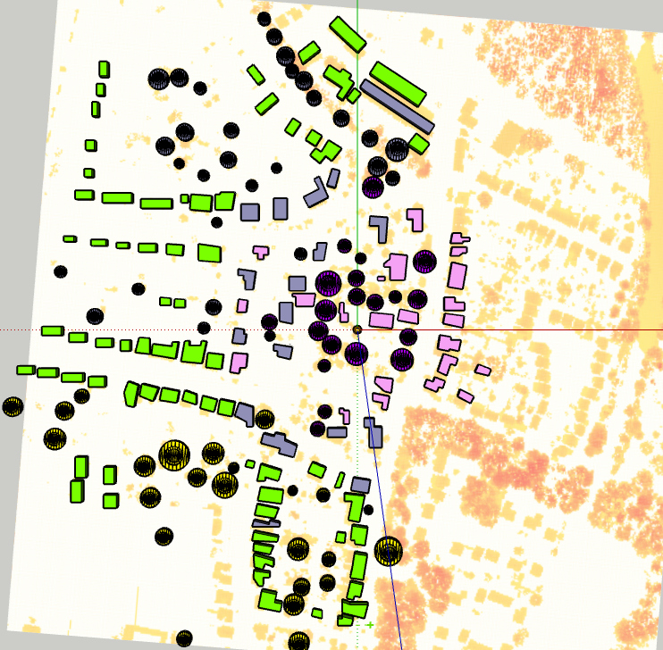
- Beside all buildings within a radius of 100m from the mill;
the buildings that have at least a green colouring (so which are
higher than DHM-rule minus 2m) are included in the CAD-model.
- Here is a bird eye's view of the resulting CAD-model (without
trees) (top is North; bottom is South; right is East; and left
is West):
Simulation without trees
using SIMSCALE
- General guidelines how to use CFD in an urban environment can
be found in this guideline
[Franke, 2007].
- As much as possible default SIMSCALE options have been used.
- Open space on: the left side (25H with H=5m); right side (10H
with H=10m); inflow side (7H with H=10m) and outflow side (10H
with H=10m).
- Turbulence model: k-omega SST and residuals < 0.01
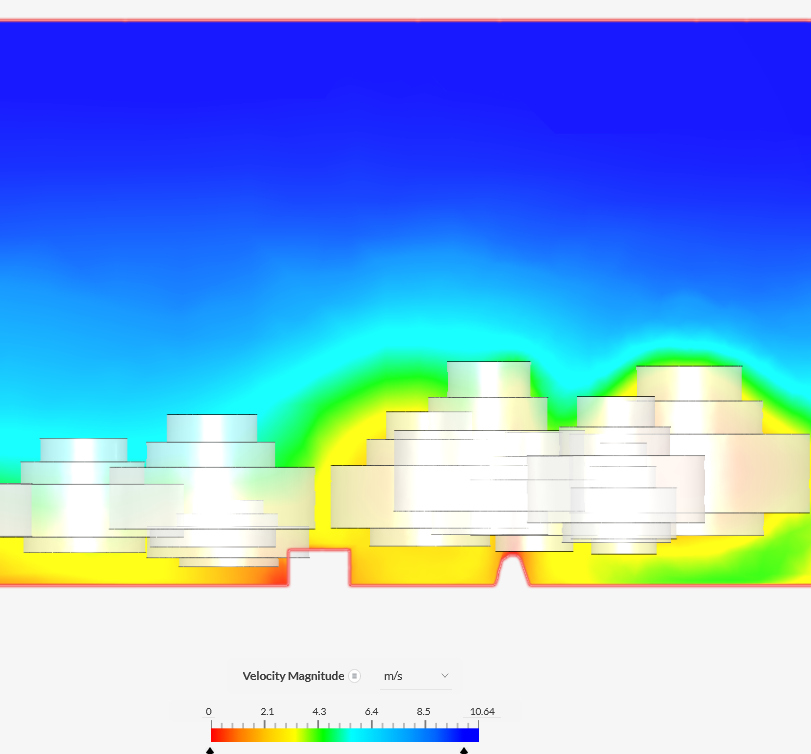
- This model (without trees) has been simulated in SIMSCALE (nl)
using an ABL for an Eastern wind of 7.1m/sec (4.6Bft) @ 10m
above ground level mill and an z0 = 1m.
CAD-model including the trees
- Including trees in SketchUp Free is not easy if using Google
Map, as one can't see the trees in Street map. A better way is
to Import the DSM height Image, which includes buildings and
trees.
- The trees are including by using the stacked-cylinder
object.
- Starting with a standard tree (15.3m high and 15.3m diameter)
in SketchUp Free.
Scale this tree by using:
Scale → Uniform Scale About Opposite Point →
enter xyz scaling
Scale → Blue Scale About Opposite Point →
enter z scaling
- At first, only trees that will affect the winds between
South-West were included and later the trees in the North-West:
Used by Stephen
Temple (in Excel)
|
Used by Victor Reijs
(in CDF)
|
NW tree is at 330deg @ 269m
|
 |
- De CAD model changes for every wind sector (steps of 15deg) in
SIMSCALE CAD mode:
- Rotated with a certain value (Transform →→
Rotate Z-axis → Rotation angle →
<value> → right click → Assign All →
Apply)
- Flow volume → input X min, X max, Y min, Y max, Z
min, Z max → Excluded parts → Select trees →
Apply
- Flow region → Hide → Select Trees →
Invert selection → Delete → Apply →
Flow region Unhide → Save as Copy
Combining the wind
speeds and directions, 1st wind rose iteration
- General guidelines how to use CFD in an urban environment can
be found in this guideline
[Franke, 2007].
- As much as possible default SIMSCALE options have been used.
- Open space on: the left side (25H with H=5m); right side (10H
with H=10m); inflow side (7H with H=10m) and outflow side (10H
with H=10m).
- Turbulence model: at start k-omega SST and at the end Realized
k-epsilon and residuals < 0.01
- Scenario 3
was used as the basis for this particular sector evaluation. In
the future a more appropriate scenario (19?) will be checked.
- In SIMSCALE we use a Forchheimer coefficient of f=0.45
[1/m] for leafed/summer trees (Ulmus parvifolia; using the
Darcy-Forchheimer
medium).
- Simulations were done for wind directions from 180 to 270deg
in steps of 15deg using the project: DSM2022 Impington.
- Input ABL wind speed is 7.1m/sec @ 10m and z0=0.5.
A lower z0 has been used (compared to earlier this
page) as the wind speed at the mill is compared to wind speed at
the Mildenhall (which is in quite open terrain).
- When measuring the calculated speed at 75%
of the sail span (75% of 9m) in a vertical sail-plane in front of the mill body
(2.7m from the centre of the mill body) with wind shaft at 15m
height, the following wind speeds (relative to Mildenhall ABL
wind speeds: u(ABL)) were calculated:
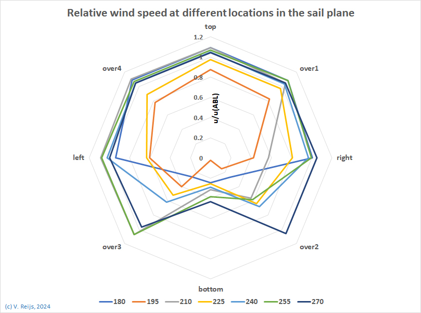
- When repeating the measurement of the calculated wind
velocities a standard deviation of some 0.2m/sec is found.
- When a sail is at its lowest point (bottom, around 8.5m),
the lowest wind speeds were calculated (due to upwind effect
of the mill body).
- The wind speeds at the highest point (top, around 21.5m) are
for most wind direction close to the Mildenhall ABL wind speed
for such heights.
- The wind speeds at the low locations (over2,
bottom, over3) is effected by buildings and trees
in the neighbourhood.
- For Impington Mill: Trees (up to 19m) have the most effect
compared to buildings (up to 8m).
- The influence of the terrain (at 15m height) within100m
upwind is as follows for each azimuth:
180
|
195
|
210
|
225
|
240
|
255
|
270
|
open
|
nearby
tree
|
open
|
far
trees
|
open
|
open
|
open
|
- For wind directions of 195 and 225deg, the wind speed at all
locations is reduced; due to respectively a nearby high tree
(around 15.5 high at a distance of some 20m) and a line of
four high trees (between 12 and 15m high at a distance between
20 and 200m).
- A few other locations were also simulated (as these could be
indicators of rotational energy or positions of sensors).
- The locations are:
- 0.4m above the mill cap: yellow (close to a former
anemometer location at Impington Mill [locA])
- avg around the
circumference of 75% of sail length
(8 averaged): green (an indicator of the mill's rotational
energy)
The dotted green line is a trendline through the calculated
values.
- avg of right and left locations of 75% of sail
length (2 averaged): blue (a simpler indicator of the mill's
rotational energy)
- in front of wind shaft: black
- Impington: red (measured by
Temple [2024])
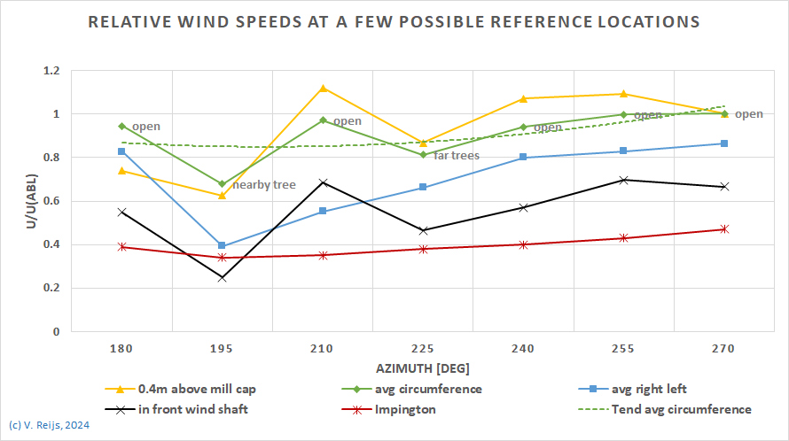
- The wind speed above the mill cap (yellow) is high compared
to ABL (due to turbulence?).
- It is expected that the average
wind speed over the circumference (green) is the best proxy for
the rotational energy available to the mill. Within the
azimuth of 180 to 270deg (the general wind direction is around
240deg), the wind speed at Impington Mill is between 60 and
100% of Mildenhall's.
- The average wind speed over the circumference (green) is
slightly higher than the average wind speed over only left and
right position (blue: at wind shaft height).
- The wind speed in front of the wind shaft (black) is low
(due to upwind effects of mill cap and/or obstructions).
- In general, all the locations have similar calculated
behaviour (like due to the high trees).
- In the future a more appropriate scenario (19?) will be checked.
Sensitivity analysis around several
parameters
Several scenarios have been simulated to see how the (magnitude of
the) average wind speed (from SW direction, with ABL's z0=0.5m)
was influenced by varying several parameters (using OFT
[One-Factor at a Time] analysis):
- related to trees:
- placemen
- height
- number
- form (stacked cylinder [sc] and cylinder [c])
- porosity (single f [sf=0.45] to multiple f [mf=0.8, 1 and
1.4])
- related to buildings
- height (incl. physical roof handling)
- related to CDF simulation
- turbulence model (k-omega SST or realized
k-epsilon);
- CDF parameter initialisation
- the height of the flow regio
- boundary layers in mesh
- the roughness of the ground
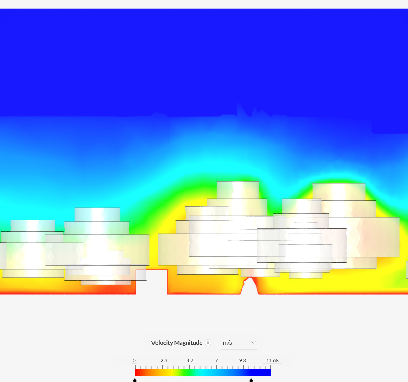
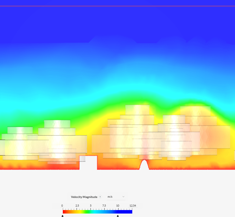
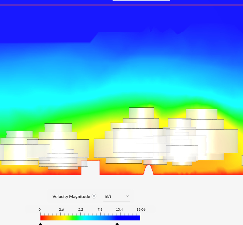
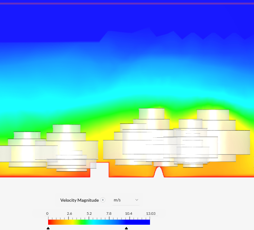
Here is an overview of these scenarios:
Scenario
|
1
|
2
|
3
|
4
|
5
|
6
|
7
|
Roof
height
|
DSM2019, midway
|
DSM2019, midway
|
DSM2019, midway
|
DSM2019, ridge
|
DSM2019, ridge |
DSM2019, ridge |
DSM2019, ridge |
Trees,
placement
|
14sc, hand, sf
|
21sc, DSM2019, sf
|
25sc, DSM2022, sf
|
25sc, DSM2022, sf
|
25sc, DSM2022, sf
|
25sc, DSM2022, sf
|
25sc, DSM2022, sf |
Turbulence
model
|
k-omega SST
|
k-omega SST |
k-omega SST |
k-omega SST |
k-omega SST |
k-omega SST |
realized k-epsilon |
flow
region
height [m]
|
40
|
40 |
40 |
40 |
40 |
40 |
40
|
Ground
roughness
height [m]
|
small
|
small
|
small
|
small
|
0.5
|
10
|
10
|
View
|
|
 |
 |
 |
 |
 |
 |
Scenario
|
8
|
9
|
10
|
11
|
12
|
13
|
14
|
Roof
height
|
DSM2019, ridge |
DSM2019, ridge
|
DSM2019, ridge |
DSM2019, ridge |
DSM2019, ridge
|
DSM2019, ridge |
DSM2019, ridge
|
Trees,
placement
|
25sc, DSM2022, sf
|
25sc, DSM2022, sf
|
25sc, DSM2022, sf
|
25sc, DSM2022, sf
|
25c, DSM2022, sf
|
25c, DSM2022, mf
|
25sc, DSM2022+10%, mf
|
Turbulence
model
|
realized k-epsilon |
realized k-epsilon
initialised
|
realized k-epsilon
initialised, boundary layer
|
realized k-epsilon
initialised, boundary layer |
realized k-epsilon
initialised, boundary layer |
realized k-epsilon
initialised, boundary layer |
realized k-epsilon
initialised, boundary layer |
flow
region
height [m]
|
100
|
100 |
100 |
100 |
100
|
100
|
100
|
Ground
roughness
height [m]
|
1
|
1
|
1
|
10
|
10
|
10
|
10
|
View
|
 |
 |
 |
 |
 |
 |
 |
Scenario
|
15
|
16
|
17
|
18
|
19
|
Roof
height
|
DSM2019, ridge |
DSM2019, ridge
|
DSM2019, ridge |
DSM2019, ridge |
DSM2019, ridge
|
Trees,
placement
|
25c, DSM2022+10%, mf
|
25c, DSM2022+10%, mf |
25c, DSM2022+10%, mf |
25c, DSM2022+10%,
mf+0.2 |
25c, DSM2022+10%,
mf+0.4 (oak)
|
Turbulence
model
|
realized k-epsilon
initialised, boundary layer |
realized k-epsilon
initialised, boundary layer |
realized k-epsilon
initialised, boundary layer |
realized k-epsilon
initialised, boundary layer |
realized k-epsilon
initialised, boundary layer |
flow
region
height [m]
|
100
|
100
|
150
|
150 |
150
|
Ground
roughness
height [m]
|
10
|
1
|
1
|
1 |
1
|
View
|
 |
 |
 |
 |
 |
Scenario
|
20
|
21
|
22
|
23
|
24
|
Roof
height
|
DSM2022, ridge |
DSM2022, ridge |
DSM2022, ridge |
DSM2022, ridge |
DSM2022, ridge |
Trees,
placement
|
25c, redo-DSM2022,
mf+0.4 (oak)
|
25c, redo-DSM2022,
mf-~0.4
|
25c, redo-DSM2022,
mf-~0.2
|
25c, redo-DSM2022,
mf-~0.45 (beech) |
25sc, redo-DSM2022,
mf-~0.45 (beech) |
Turbulence
model
|
realized k-epsilon
initialised, boundary layer |
realized k-epsilon
initialised, boundary layer |
realized k-epsilon
initialised, boundary layer |
realized k-epsilon
initialised, boundary layer |
realized k-epsilon
initialised, boundary layer |
flow
region
height [m]
|
150
|
150
|
150
|
150
|
150 |
Ground
roughness
height [m]
|
1
|
1
|
1
|
1
|
1
|
View
|
 |
 |
 |
 |
 |
The scenarios are:
- The trees (Ulmus parvifolia, f=0.45,
modelled as stacked cylinders; sc) were positioned by hand, say
within 10m of their actual position (the ground plane from
Google Map does not include trees).
- Now DSM2019 was included as ground plane and thus trees are
positioned more accurately. Some trees were missing, perhaps
because it was a DSM from 2019.
- The DSM2020 was included as ground plane and the height of the
trees was adjusted (first echo, so they were on average some 2m
higher than in scenario 2).
- The height of buildings is up to ridge roof height; on average
some 30% higher then when using the average roof height.
Remember that not all roofs are perpendicular to the wind
direction!
- The ground layer has a roughness height of 0.5m.
- The ground layer has a roughness height of 10m (=20*z0
[Dong, 2015, page 11004]; Rasaders).
- The turbulence model realized k-epsilon, which should
be better for turbulence in this mill environment [pers. comm.
fvgool, 2024].
- The flow region height is 100m. In the earlier scenarios this
flow region height was too small, as it should be at least 6*H
(and H=16m in this case). Ground Roughness heights of 3, 5 and
10m did not work (Gauge pressure field started diverging).
Adding the necessary boundary
layer at ground level (and perhaps general Initialisation) looks
to solve this issue (scenario 11).
- Several parameters were initialised (gauge pressure, speed, k,
epsilon, and potential flow initialisation enabled).
- The boundary layer in the mesh was included for the ground
level (this is essential for a good mesh)
- Increased Roughness height of ground
level to 10m
- Changed stacked cylinder (cs) trees to one-cylinder (c) trees,
plus the buildings were sometimes merged to improve the meshing.
- The f (Forchheimer coefficient) was made depending on the tree
height (mf: between 0.4, 0.6 and 1.0).
- Increased the height of all stack cylinder trees (sc) with 10%
(which is closer to the GE and DSM values)
- With increased height of trees: but now with c-trees
- Back to roughness of 1m for the ground layer (as the roughness
of 10m also acted on/for the houses, which is not correct)
- Changed the height of the flow region to 150m (6*H; as the
trees are heightened to H=22m in scenario 14)
- Increased the f with 0.2 (so f is now: between 0.6, 0.8 and
1.2)
- Increased the f with 0.2 (so f is now: between 0.8, 1.0 and
1.4.
Looking at optical porosity of the 5% (much denser than leafed Quercus
robur which ihas an optical porosity of around 15%)
this gives an f of 0.9.
- Re-measured the height of buildings and trees in DSM2022. In
general an increase of 3%
Buildings' height is referenced to ground level. The trees'
heights have been referenced to mean sea level (MSL) relative to
mill's base, for Impington the trees' height from ground level
are a little higher, but this difference has not been included
('compensated'), because the trees were proxied by a cylinder (ellipsoid form would
have been better, but I was not yet able to model that).
- Reduced f to a value for 20% optical porosity: f is now
between 0.2, 0.4 and 0.6 (to determine the sensitivity to
porosity or f)
- Reduced f to a value for 40% optical porosity: f is now
between 0.1, 0.2 and 0.3 (to determine the sensitivity to
porosity or f)
- Changed f to a value closer to a Quercus robur
tree (15% optical porosity [Braun, 2024, Figure 3]: f is now
between 0.45, 0.65 and 1.0)
- The cylinders have been replaced with
stacked cylinder (sc) models for trees.
- Changed stacked cylinders (sc) trees to
an ellipsoid (e) trees and rectangular boxes with gabled roofs.
The ellipsoid trees do not yet calculate in SIMSCALE, but it is
expected that the wind speed will not change significantly
The gabled roofs do not yet calculate in SIMSCALE, but it is
expected that the wind speed will be slightly lower.
Remark: The STL file
made by SketchUp has problems. Advised to use STEP or
Parasolid. Onshape could
be used. I am investigating this.
- Changing the mesh-Fineness. This has been done at another
mill-simulation, which showed low dependency (<10%):
and the higher the Fineness the lower the speed (at least in
that example). This is of course depending on the whole 3D
model, so one needs to check this actively!
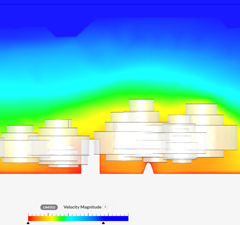
The resulting (magnitude of the) averaged windspeed (relative to the
ABL speed at the same height) over the wing rotation surface can be
seen below.
In general CFD will not be 100% accurate. But 10% speed accuracy
should be reachable with a reasonable effort [Pirkl, 2020]. So the
below relative speeds have a standard deviation of around 4%
and relative energy has a standard deviation of around 3%. Beside
this, the location of measuring in the 3D environment also does map
the real location of the anemometer.
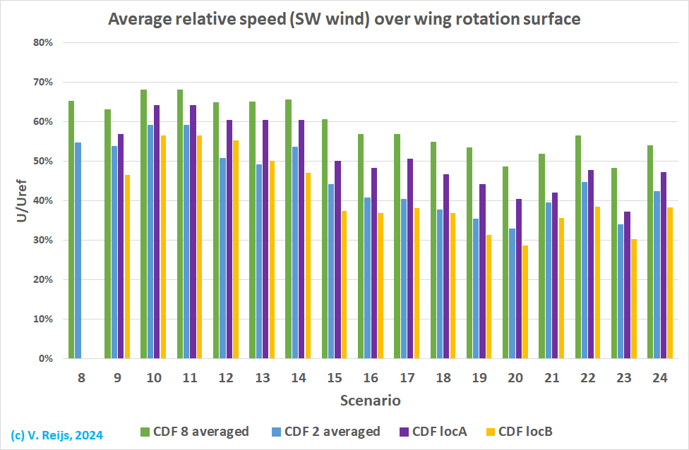
Relative
speed
|
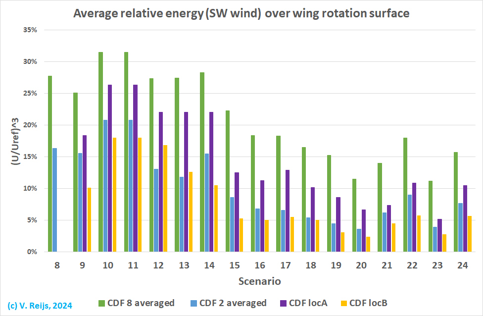
Relatieve
energy
|
 |
 |
Other observations can be deducted:
- The 8 averaged wind speed (green) is calculated by
using every 45 degrees of the wing rotation surface; while the 2
averaged (blue) is only done for the left and right
position of the sails (this is the
'recommended' wind speed position). There is some 14%
difference between the two. And if we do not measure at left and
right but 1m above left and right; both averages are
close. So, it might be good to put anemometer(s) at 1m above the
left and/or right sail position.
Remark: it is proposed to change the
definition of this 'recommended' position.
- Increasing the height of the buildings, deceased the wind
speed at shaft height (scenario 3 and 4).
This is expected as the higher buildings will provide more
blockage. It is not yet known if one should use ridge height or
average roof height.
Some simulations were done to determine which effective height of a roofed building is
most representative, see for instance at Abohela [2013].
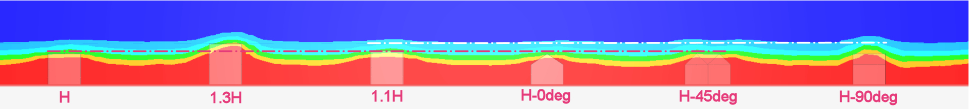
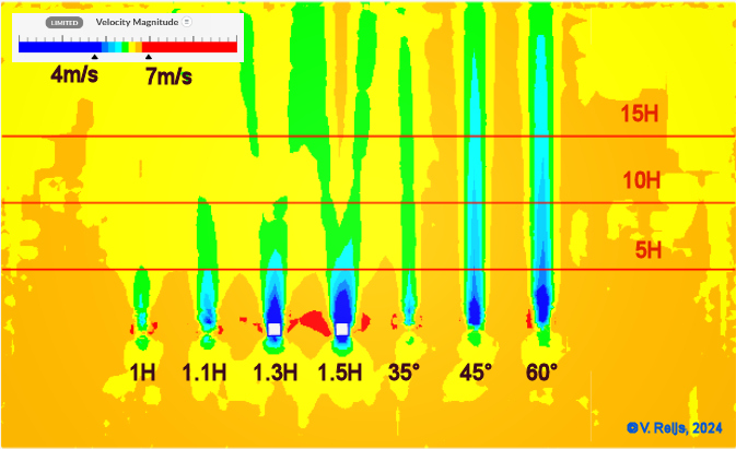
At a distance of 30m (6H, above the cavity)
and roof sloop of 35deg (American 'standard'
slanted roofs are between 14 and 37deg) and the cube is
6*6*6m=1*1*1H): A 90deg turned roof looks to be more or less
equivalent to a cube of around 1.1H. A 45deg turned roof looks
to be more or less equivalent with the original cube of 1H. So
perhaps with an average wind direction, a heightened cube of
1.05H (averaged over 1 and 1.1H) might be prudent.
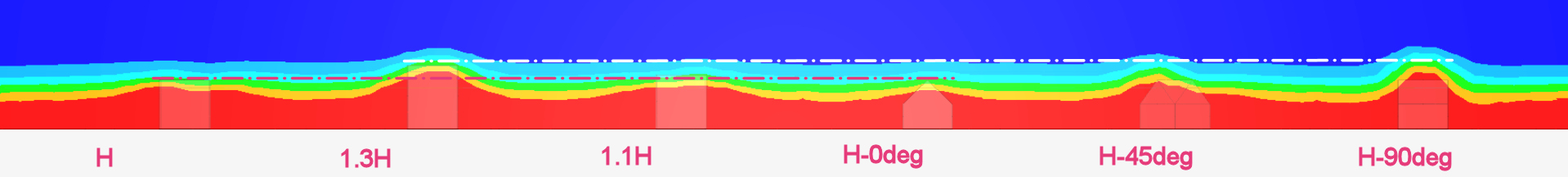
At a distance of 30m (6H, above the cavity)
and roof sloped at 45deg (close to the common roof slope seen
in The Netherlands between 40 and 60deg; while in the UK common roof slope is
between 30 and 50deg) and the cube is 6*6*6m=1*1*1H): A
90deg turned roof looks to be more or less equivalent to a cube
of around 1.3H high. So perhaps with an average wind direction,
a heightened cube of 1.15H (averaged over 1 and 1.3H) might be
prudent.
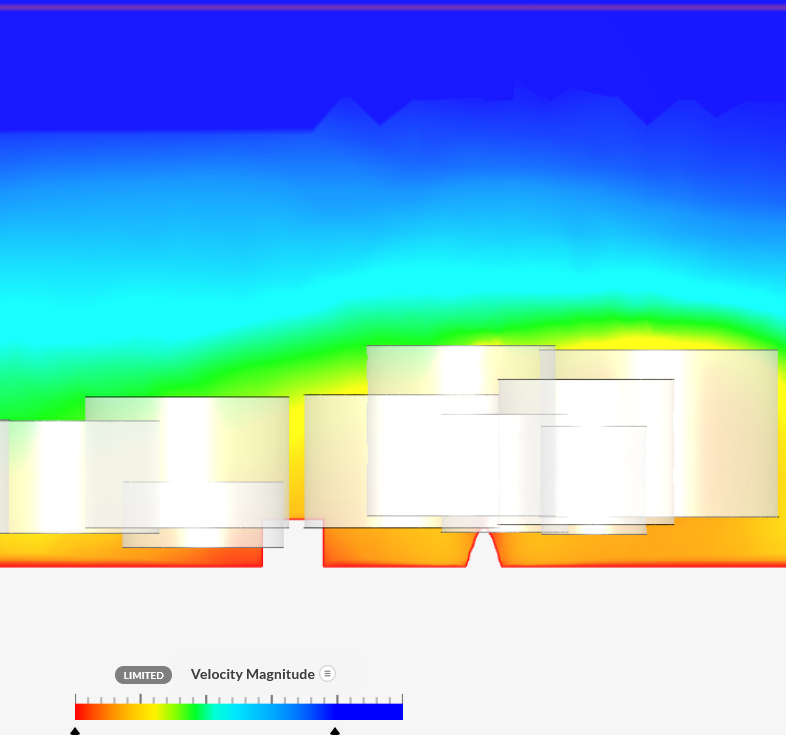
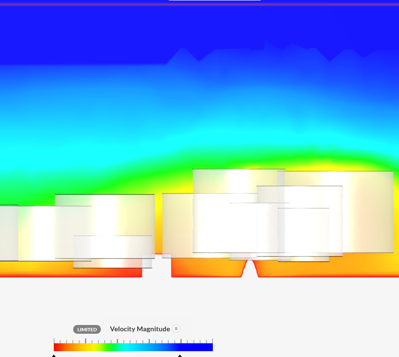
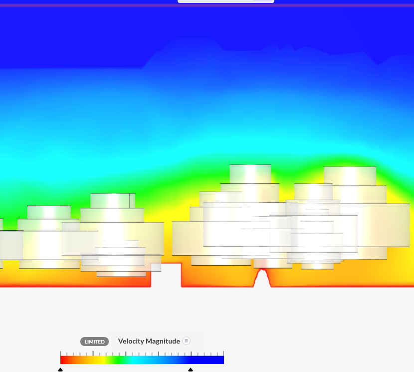
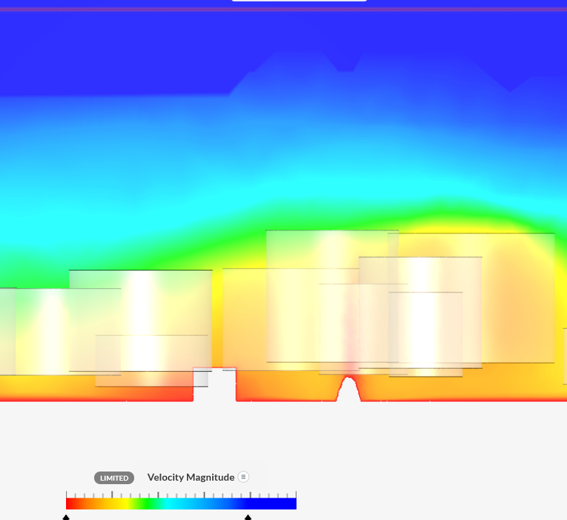
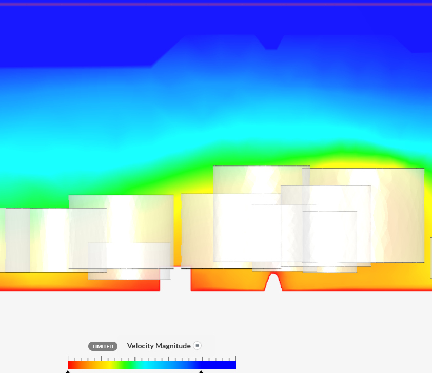
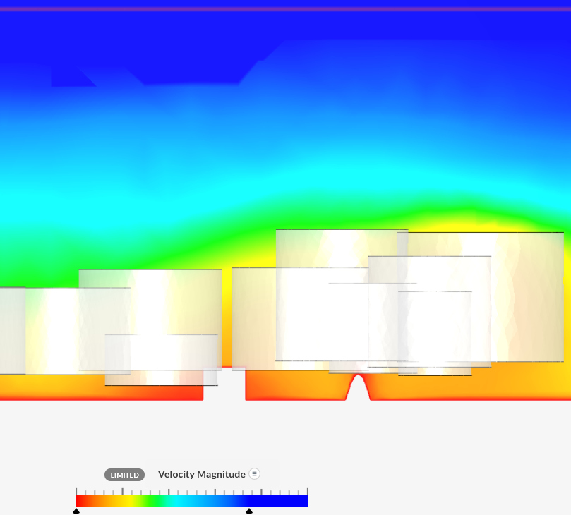
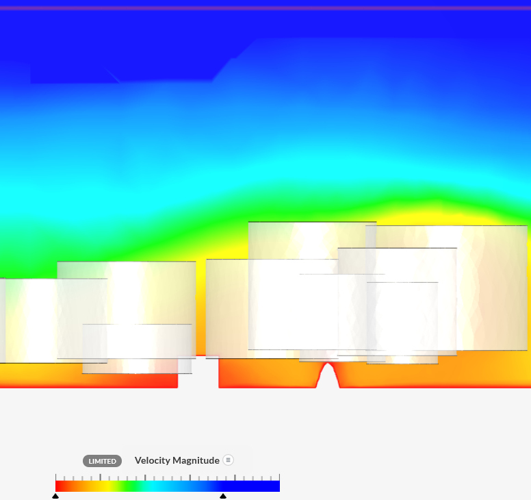
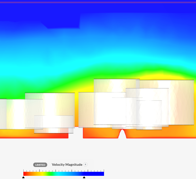
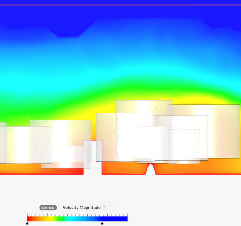
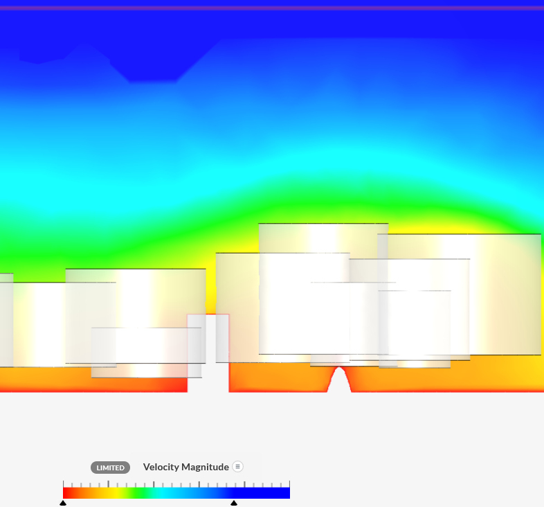
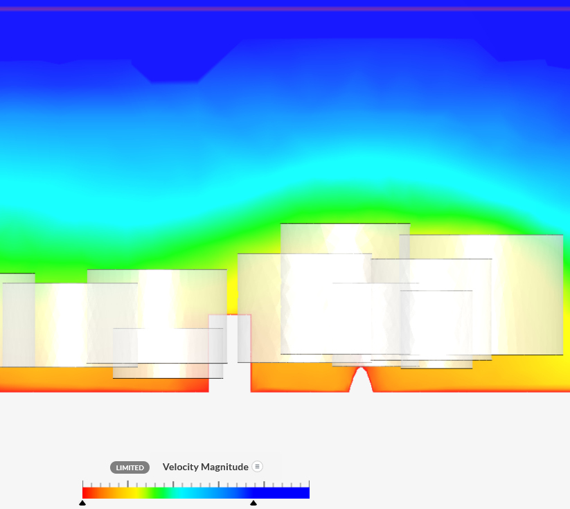
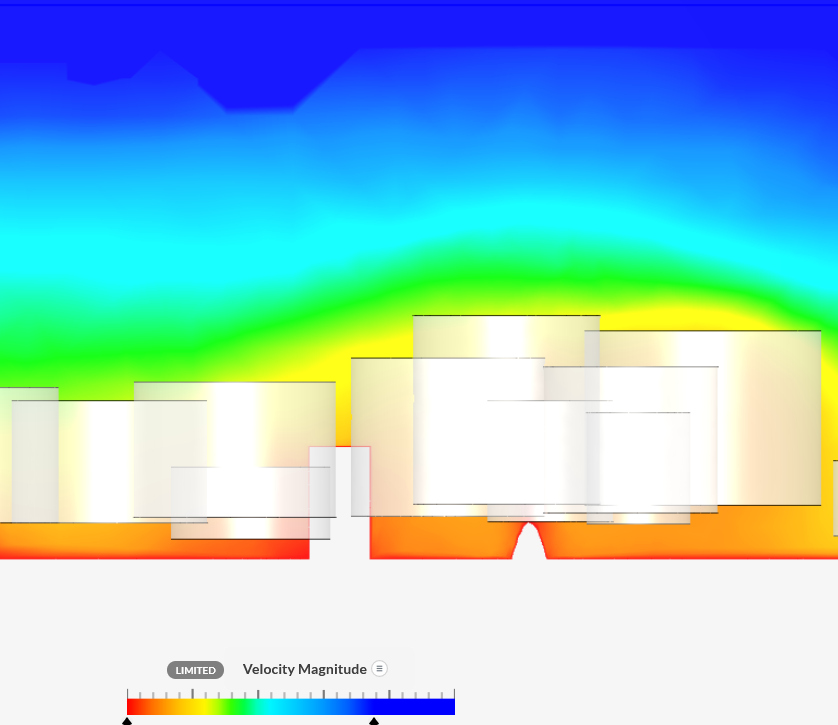
The above pictures are though not that simple. It looks that a
roof slope (all ridges are at 6m) has a more lasting reduction
of the speed then the height of a rectangular box (the speed is
shown at a height of 7.5m):
Looking at this, we might need have to include roofs in the
simulation (which is of course not a real problem in a CFD).
This would then also solve the issue of the wind direction in
relation to the ridge direction.
Stephen Temple used flat roof buildings (more likely fences) at
height of 1.3H of the ridge height.
Remark: incorporating the roof form can
be important in a CFD (certainly for nearby buildings).
- A round roughness height of 10m (=20*z0
[Dong, 2015, page 11004]; Rasaders), this
increased the (magnitude of the) wind speed (scenarios 4, 5 and
6 & scenarios 9 and 10).
Roughness height increases the turbulence and this will also
increase the speed.
- Increasing the height of the flow region to 100m, this
decreased the wind speed at shaft height (scenario 7 and 8)
This is expected as the lower flow region will return the wind
downwards and this increasing the wind at shaft height. One
needs to align with normal CFD modelling rules: height flow
region > 6Hmax (Franke, 2007, section 5.1.1). In
our case Hmax = max(Hbuilt, Htree)
= 16m.
So important to have the height of the flow region at least 6Hmax
(Franke, 2007, section 5.1.1).
- The scenarios the velocities (@ 2 averaged) are
relatively insensitivity to: number of tree, tree form, the
height of buildings; ground roughness, turbulence model and
mesh.
- With height flow region of 40m (scenarios 1 to 7) have a
standard deviation of ~6%
- With height flow region of 100m (scenarios 8 to 12) have a
standard deviation of ~3%
- The height of the trees will decrease the wind speed: 10%
height (on average 120cm) increase gives some 5% speed
decrease (scenario 11<->14 and 13<->15).
IMHO the 24th scenario
would be closest to reality.
Comparing the parameters in formula,
Excel and CFD
Parameter
|
Formula
DHM
|
Excel
ST
[2004]
|
CFD
VR
|
Buildings
|
|
location of buildings
|
thin long
obstacle,
obvious
obstacle,
x>15*H.
H>10*z0
|
1 to 3
obstacles
per sector |
3D objects
|
|
form of buildings
|
H<3*z
|
HExcel=1.3*HGE
is default
|
yes
|
Trees
|
|
location of trees
|
no
|
yes
|
yes
|
|
form of trees
|
no
|
HExcel=1.3*HGE
is default
|
yes
|
|
porosity of trees
|
no
|
yes
|
yes
|
Mill
|
|
form of mill
|
z within reason
|
z within reason |
yes
|
Landscape
|
|
Buildings/trees
|
formula
|
here
|
here
|
Underlaying
principles
|
|
flow area dimensions
|
implicit
|
implicit |
hflow>6*Hmax
|
|
boundary layers
|
implicit |
implicit |
roughness
ground layer
|
|
initialisation
|
implicit |
implicit |
optional
|
|
turbulence model
|
implicit |
implicit |
k-epsilon
|
|
'decay' rate
|
n
(omitted H/z0
dependency)
|
n= 50
is default
(omitted
H/z0
and SpeedFactor
dependency) |
implicit
|
Output
|
|
freedom of
measurement point
|
no
|
no
|
yes
|
|
wind speed
|
limited (90%,95%) |
yes
|
yes
|
|
wind direction
|
no
|
no
|
yes
|
|
wind energy
|
limited (73%,86%)
|
yes
|
could be added
|
|
turbulency intensity
|
no
|
no
|
yes
|
Configuring ABL
|
|
z0t
|
implicit
|
3m
is default
|
yes
|
Comparing Impington Mill's
anemometer measurements with meteorological stations and CDF
Average windspeeds (m/sec) around Impington
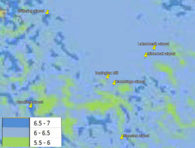
Looking at the average windspeed, the airport locations of
Cambridge, Mildenhall, Lakenheath and Wittering could be ok for
Impington Mill.
It is understood that meteorological station Cambridge speeds are
not fully correct (seem to be interpolation of a few data points),
so for now they are not used (a pity as this location is close to
Impington).
In several (Dutch) reports, we see the use of IDW (Inverse distance weighted: Apaydin, 2004, Section
5.1), which use the average of three meteorological stations.
Sluiter [2012, Section 4.5] and Stepek [2011] advise IDW for
interpolation of the wind speed at a certain location.
Remark: Is IDW a good methodology
to determine the local wind speed, or is (C)K(S/D) better?
ABL profile
The Atmospheric Boundary Layer (ABL) profile is logarithmic. The
speed U is in the form of [Wieringa, page 63]:
Uz = Uref*ln(z/z0)/ln(zref)/z0)
and z>10*z0
If one wants to determine the speed at location B when speed is
known at location A (each with a different zo); one has
to convert the speed at location A with zoA to 60m (a
common height where the speed is quite independent of zo);
and then convert this 60m speed to the speed at location B with zoB
[Wieringa, page 65]. So using the above formula twice;-):
UB = UA*ln(60/z0A)*ln(zB)/z0B)/(ln(60/z0B)*ln(zA)/z0A))
and zx>10*z0x
Error analysis
Looking at wind speed measurements at Mildenhall and Impington
The error in the speed ratio Impington/Mildenhall (if this ratio
is around 0.5) is almost independent on the standard deviation of
the Mildenhall. The error of Impington speed is thus leading.
The standard deviation of the anemometer (ecowitt; with an
accuracy: <10m/s, +/-0.5m/s; ≥10m/s, +/-5%) is
around 0.5m/sec @ 4m/sec. The standard deviation of the Mildenhall
station is around 0.5m/sec @ 8m/sec. Not knowing the correct
reference meteorological station cn provide a systematic error of
say 0.5m/sec @ 8m/sec.
This results in a standard deviation in speed ratio (@ ~0.5) of
~0.05 and a systematic error of + or - ~0.03. So in total ~0.06
Looking at wind direction measurements at Mildenhall and
Impington
The standard deviation of the wind directions specified by ecowitt
is 15deg, something
similar can be deducted from the wind direction spread of
Mildenhall and Impington:
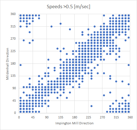
Both the Mildenhall meteorological station as the Impington
weather station look to have a standard deviation of around
15deg (135/6/sqrt(2)).
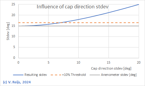
The standard deviation of
wind direction for Impington is also determined by the standard deviation of the
cap direction measurements. A correctly calibrated
magnetometer can be around 2deg. So this is small compared ot
the 15deg from the anemometer. But the magnetometer is not
alwasy easy to calibrate (like in the Dutch windmills, as no
automatic turning is done). If we allow an extra 10% increase
due to this magnetometer standard deviation, we can allow for
a standard deviaiton of around 7deg for the magnetometer.
Looking at ABL and simulation at Impington
In general, CFD will not be precise. But 15% speed accuracy should
be reachable with a reasonable effort.
The standard deviation of CDF speed simulation (15% of
4m/sec=0.6m/sec); measurement point location error (0.25m/sec) and
error measurement (0.2m/sec) is around 0.7m/sec @ 4m/sec. The
standard deviation of the ABL itself is quite low, sat 0.1m/sec.
This results in a standard deviation in speed ratio (@ ~0.5) of
~0.06 due to CDF itself.
Beside this partial CDF standard deviation, there is variability
due to the variability or unknown of porosity. Assume a standard
deviation for the porosity of around 10% and this results in a
partial standard deviation of 0.03 in the speed.
Combining this with the 0.06 it becomes (sqrt(0.06^2+0.03^2)): 0.07
The standard
deviation of the wind direction is around 0deg.
Comparing the
measured and simulated speed ratios
Comparing wind speed ratios will be done at locA and locB.
As there is no real ABL regime at these anemometer locations it is
not opportune to use the ABL function to determine the speed at
another height (like wind shaft).
See also Beljaars (1979, page 2):
"Tussen de obstakels, die de windruwheid [lengte] bepalen, valt
weinig te zeggen over deze [logaritmische] hoogteafhankelijkheid."
("Between the
obstacles that determine the roughness length, there is
little to say about this [logarithmic] height dependency)
We though can assume that the atmosphere
at the meteorological stations is much closer to an ABL, so we can transform the 10m
speed to locA or locB speeds.
As the measurements will happen many times (aka averaging), the
resulting standard deviation will be reduced with sqrt(n). As the
n per sector will be large, the influence of this standard
deviation on the comparison will be small. The influence of
systematic error stays.
The standard deviation of the comparison of the two ratios is
~0.07 (which is due to the standard deviation of the simulation)
and a systematic difference of + or - 0.03 (most likely a plus).
Influence of wind direction variability
on the comparison of measured and simulated speeds.
When comparing the measured speed with the simulated speed it is
important to take into account the variation (standard deviation,
which is around 15deg) of the wind direction of the measured wind
speed. This means that to compare the measured wind speed at a
certain direction with the simulated windspeed at that direction;
one needs to combine simulated speeds of directions of say up to
plus or minus 25deg.
Using Temple's measurements at Impington
Mill
The anemometer was at
around 17m and behind the sails and in front of middle of mill
cap (locA@17m)
The measured averaged wind speed (m/sec) of Impington Mill (black:
Anemometer) and meteorological station Mildenhall (grey: Open
Fields) are provided for summer time (May to September and
averaged over 30 years) in below figure (Temple, 2024, @ 21:36).
All speeds are referenced to 15m (shaft height), by using for both
statios a z0 of 3m.
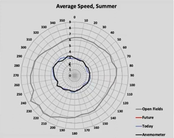
The behaviour of the lines
could be seen as slightly comparable (a dip around 195deg): the
dotted green line (trendline of avg. of circumference) matches
the form of Impington line.
The Impington Mill wind
speed (locA@15m) at
wind direction of 225 deg is around 38% (=3/8) (standard
deviation ~6%) of
the Mildenhall values at Summer
months
Using smartmolen data
At present (May 2024) the Impington Mill weather station is at the
back of the fantail frame, at more or less the same level as the top
of the mill cap: 16m (locB@16m).
Here is average wind speed data from Impington Mill weather station (black),
meteorological stations (Mildenhall: orange, Lakenheath: grey and
Wittering: green); and the ratio between Impington Mill and
Mildenhall (dotted orange) over part of Summer Month (May
1st to 18th). All speeds are referenced to 16m, by using a z0
of 0.25 for Mildenhall and other meteorological stations.
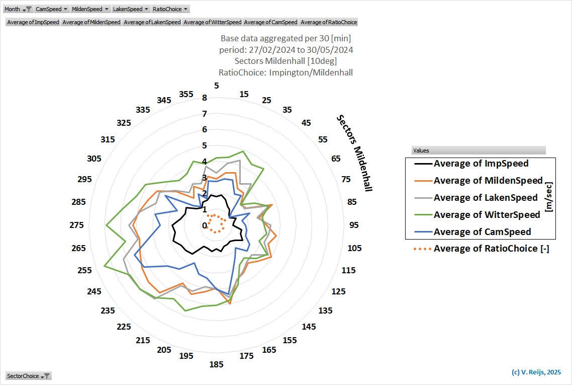
The Impington Mill wind speed (locB@16m) at wind direction of 225
deg is around 43% (standard
deviation ~6%) of the Mildenhall values at
part of May (Summer month).
Simulated speeds
Below is an overview of the simulated CDF speeds (wind direction
of 225deg) for several locations using scenarios 1 to 24:
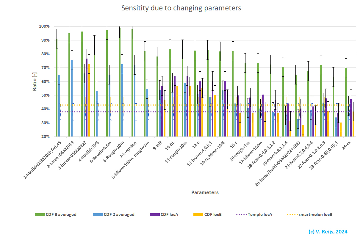
Scenario 24 is using DSM2022 tree and building heights and f
close to optical porosity for Quercus robur trees:
The Impington Mill wind speed (locA@17m) at
wind direction of 225 deg is around 47% (standard deviation
~7%) of the Mildenhall values at
Summer month.
The Impington Mill wind speed (locB@16m) at
wind direction of 225 deg is around 38% (standard
deviation ~7%)
of the Mildenhall values
at Summer month.
Combining the wind speeds and
directions, 2nd wind rose iteration
This is the second wind rose iteration after the first wind rose
determination.
Some general conditions:
- LocA is the location of the anemometer used by Steven
Temple (above the shaft at the front: 17m height)
- LocB is the location of the anemometer used by
smartmolen (left on the fantail frame: 16m height)
- LocC is the possible location of the future anemometer
used by Steven Temple (infront of the shaft: 15m height). This
is not further evaluated in the below.
- The z0 at Mildenhall (the reference location) is
0.25m [Many trees, hedges, few buildings; Manwell, 2009,
Table 2.2].
The reference speed has been corrected for the height of locA,
locB and locC.
- The z0 around Impington Mill would be
around 1.5m [Suburban; Manwell, 2009, Table2.2].
This has no effect as the wind of the reference location
(Mildenhall) is the only one that is height compensated to the locA
or locB.
- A Impington Mill fictive z0 (which would be
around 11m) is also not used to correct the locA,
locB and locC to the shaft height (as the wind
profile near the mill is not likely a power law curve).
- A z0 of 0.5m was used for the inlet ABL speed of
the CDF for all wind directions.
- Height of buildings is as in the DSM2022 (from ground level)
and a house is rectangular box with height of the roof ridge
- Height of trees is as in the DSM 2022 (from base of mill
level). Not at ground level as the trees are modelled as
cylinders, while an ellipsoid should be better (and their
effective height would be slightly smaller).
- A random mix of oak and beech trees was used (average optical
porosity around 0.2)
Depending on height resulting in trees with f=0.25, 0.65, 0.85
or 1.
- The speed ratio has been probability
weighted of speeds at the mean wind direction and two wind
direction sectors below and above this mean (due to the standard
deviation of the wind direction: +/- 15deg).
- The purple dotted curve is averaged over a long period (whole
summer: 5 months)
- The yellow dotted curve is averaged over a short period (1.5
months)
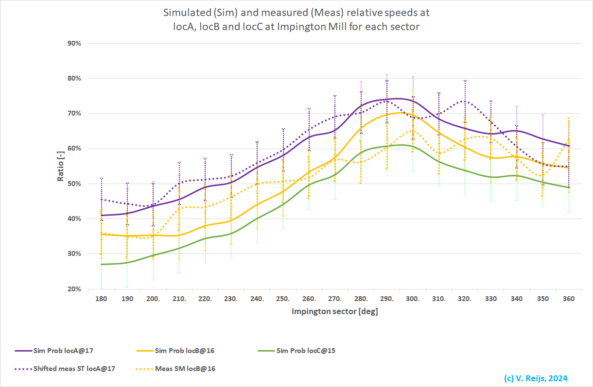
The wind rose for Impington Mill (between 180 and 360deg over
West) can be seen below:
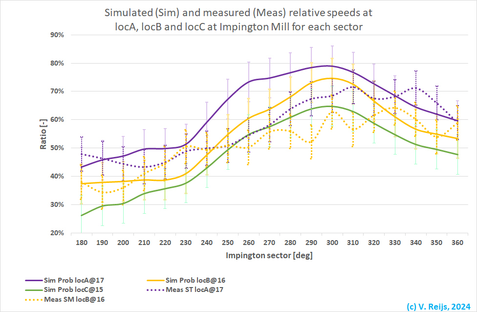
What can be seen in this graph:
- The simulated ratios of locA (continuous purple), locB
(continuous yellow) and locC (continuous green)
have a similar form.
The continuous yellow curve is lower, as locB is in a
more sheltered location (left behind the cap).
- The peak of the continuous yellow curve is at a slightly
higher wind direction than locA.
This is perhaps because the anemometer is left of the cap
middle.
- The measured ratios at locA (dotted purple) and locB
(dotted yellow) have a similar form.
The dotted yellow curve is lower, as locB is in a more
sheltered location (left behind the cap).
- The measured curves look to be slightly moved to a higher wind
direction (say 30deg).
Don't know a reason: the simulated one use the True North (from
DSM2022). I assume the North direction of the anemometer is also
correctly set (there is no real difference in direction [some
10deg] for instance between Impington Mill and Mildenhall).
- For wind directions of 280 and 300deg, the terrain looks to be
relatively open, even close to the mill (compared to the other
wind directions).
- For wind directions between 240 and 320deg, the measured
ratios look to be significantly lower (on average ~12%) than the
simulated speed ratios.
- Additional 30 trees and 25 buildings. This had a slight
increase (2%)
- z0 = 0.5m (Forest and woodland) was used
for the inlet ABL speed of the CDF (using an averaged z0).
The western terrain is quite flat (agricultural: Crops;
Manwell, 2009, Table2.2) so a differentiation is needed
regarding z0 and wind direction (with the blue
rectangle is the terrain that is included in the CDF).
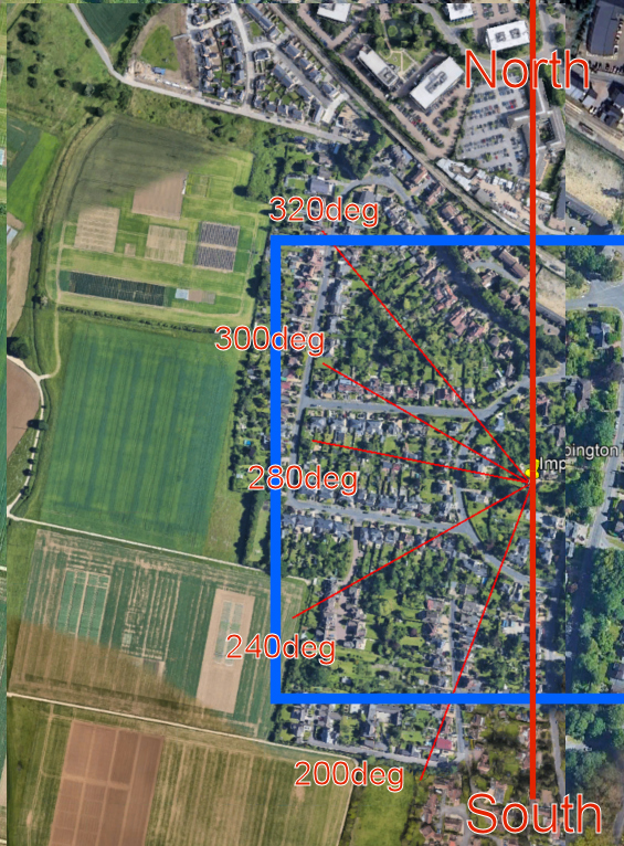
Tests (at wind direction 260deg) have been done with z0
= 0.05 (Crops), 0.1 (Few trees), 0.25 (Many
trees, hedges, few buildings), 0.5 (Forest and
woodland), and 3m (Centres of cities with tall
buildings).
Speed ratio changes were seen of around: -13% for z0
= 0.05m; -7% for z0 = 0.1m; -2% for z0
= 0.25m; and +90% for z0 = 3m.
- So a z0 = 0.05m would be better then z0
= 0.5m for the wind directions 240 to 320deg.
- In general, the measured ratios are om average lower (some 5%)
than the simulated ratios.
Combining the wind speeds and directions, 3rd
wind rose iteration
The only change with regard to the 2nd wind rose iteration is that
the inlet z0 has been decreased to 0.05m between 200
and 320deg.
Some general conditions:
- General guidelines how to use CFD in an urban environment can
be found in this guideline
[Franke, 2007].
- As much as possible default SIMSCALE options have been used.
- Size of the flow region: the left side (25H with H=5m); right
side (10H with H=10m); inflow side (7H with H=10m) and outflow
side (10H with H=10m).
- Turbulence model: Realized k-epsilon and residuals < 0.01
- LocA is the location of the anemometer used by Steven
Temple (above the shaft at the front: 17m height)
- LocB is the location of the anemometer used by
smartmolen (left on the fantail frame: 16m height)
- LocC is the possible location of the future anemometer
used by Steven Temple (in front of the shaft: 15m height). This
is not further evaluated in the below.
- The z0 at Mildenhall (the reference location) is
0.25m [Open landscape, crops of varying height,
scattered-shelter-
belts; Wieringa, 2001, Table 5.2].
The reference speed has been corrected for the height of locA,
locB and locC.
- A 'target' z0t can be chosen to compare the
simulated with the measured values of a past/present/future
Impington Mill region:
- To minimise the difference between speed
measurements and simulations (in the range 170 to 370deg) of locA
and LocB: a z0t of 0.39m is needed for
the Impington Mill region.
- The z0t around Impington Mill region is theoretically
expected to be around 1m [Mature forests, low-rise
built-up areas; Wieringa, 2001, Table 5.2].
Remark: This theoretical z0t
should be closer to the 0.39m, or not? So is my assumption
wrong for this theoretical terrain?
- The z0t around the at Impington Mill-construction-time
region would be around 0.25m [Open landscape, crops of
varying height, scattered-shelter-belts; Wieringa, 2001,
Table 5.2]. This is the z0 of the Mill without the
town buildup.
- A z0t around a to-be-checked Impington
Mill region can be any resonable value (between 0.01
[Cultivated area, low crops, occasional obstacles] and 2m
[City centre, big forest with large clearings]). So one can
compare the effects due to different terrains.
Remark: to do this one should use a
reference ABL (with a certain z0)
and then go to 60m and then get a new uref in
ABL formula for the different z0.
In the below: Only the z0 was changed
and not the uref. In the next iteration this
should be rectified.
- A Impington Mill fictive z0
(which
would be around 10m) is not used to correct the locA,
locB and locC to the shaft height (as the wind
profile near the mill is not likely a power law curve).
- A z0 of 0.05m was used for the inlet ABL speed of
the CDF for wind directions in the range 200 and 320deg. The
effect of this for the range 200 to 230deg is small (due to the
high trees in these directions near the mill)
- A z0 of 0.5m was used for the inlet ABL speed of
the CDF for wind directions outside the range 200 and 320deg.
- Height of buildings is as in the DSM2022 (from ground level)
and a house is rectangular box with height of the roof ridge
- Height of trees is as in the DSM 2022 (from base of mill
level). Not from ground level as the trees are modelled as
cylinders, while an ellipsoid should be better (and their
effective height would be slightly smaller).
- A random mix of oak and beech trees was used.
Average optical porosity around 15%: depending on height
resulting in trees with f=0.25, 0.45, 0.65, 0.85 or 1.
- The speed ratio has been probability weighted of speeds at the
mean wind direction and two wind direction sectors below and
above this mean (due to the standard deviation of the wind
direction: +/- 15deg).
- The purple dotted curve is averaged over a long period (whole
summer: 5 months)
- The yellow dotted curve is averaged over a short period (2.5
months)
The wind rose for Impington Mill
(between 180 and 360deg over West) can be seen below:
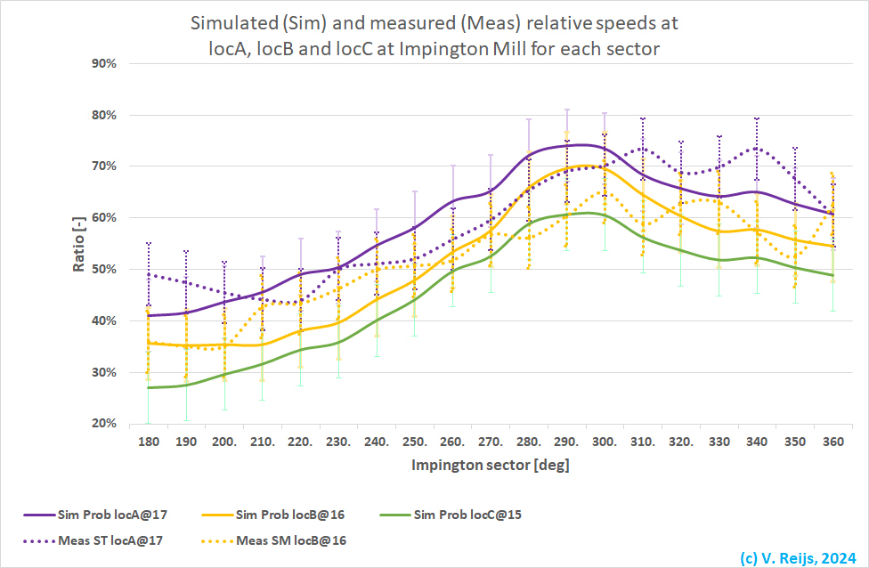
What can be seen in this graph:
- The simulated ratios of locA (continuous purple), locB
(continuous yellow) and locC (continuous green)
have a similar form.
The continuous yellow curve is lower, as locB is in a
more sheltered location (left behind the cap).
- The measured ratios at locA (dotted purple) and locB
(dotted yellow) have a similar form.
The dotted yellow curve is lower, as locB is in a more
sheltered location (left behind the cap).
- If one simulates the speeds at the
same longitude and latitude as locA, locB and locC,
and converting the speeds at the heights @17 and @16m of these
locations to a 15m height; one would need a fictive z0
of around 11m.
- Wind direction shift:
The measured (dotted) purple curve
looks to be slightly moved to a higher wind direction (say
20deg).
- The simulated ones use the True North (from DSM2022). I
assume the North direction of the anemometer is also correctly
set.
- There does not look to be a real difference in direction
[some 10deg] for instance between Impington Mill and
Mildenhall.
- In above the wind direction was taken the same as at the
inlet of the flow region. This is not fully true (obstacles
will have changed the wind direction at the mill). When
looking at the simulated wind directions at the locs,
the difference with the inlet wind direction is on average
between 1 (locA and locC) and -3 degrees (locB;
which is left behind the mill).
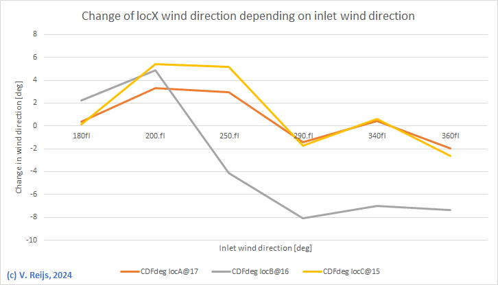
The standard deviation of the measurements (15deg) is three
times as large as the change_in_wind_directions' standard
deviation.
- Another (additonal) reason could be due to the dependency of
the measured wind direction on the positoning of two devices:
the magnetometer (to determine the cap direction) and the
weather stations wind direction (relative to the cap
direction). The magnetometer was rotated on the eye to the
sheer beam and the weather station on the shaft. So an error
of some 20 to 30deg might be possible.
If the measured speed is shifted 20deg in shrinking direction, we get
the following graph:
- For wind directions of 280 and 300deg, the CDF terrain looks
to be more open (given higher speeds) than seen in the
measurements.
- This all could also be because of the above angle
shift.
- Here is an overlay of Google
Earth and the SketchUp model.
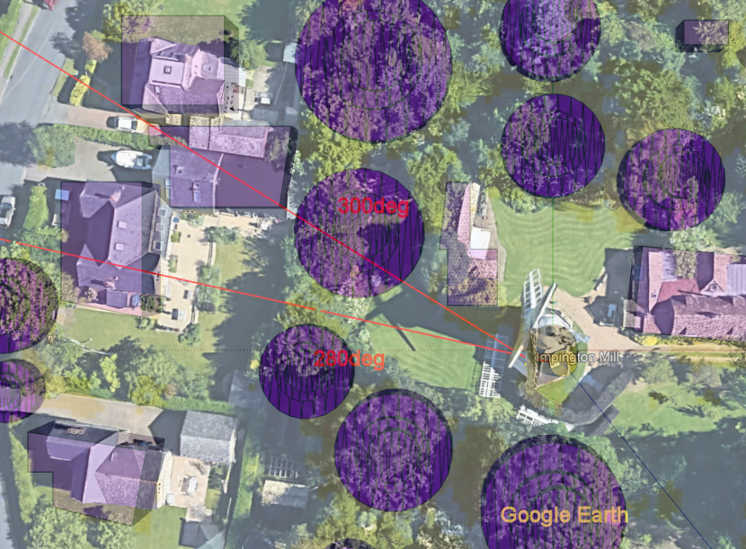
One can see that there is in the SketchUp model an opening
around 280deg.
Remark: In
the next iteration this opening between trees at 280deg will
be rectified.
- The continuous (simulated) and dotted (measured) curves of the
same color are within each other's standard deviation (except
for this 280 and 300deg wind directions of locB, see above).
- For locA and locB the simulated ratio
(continous curve) migth be systematicly higher then the measued
ratios (dotted).
The average difference between the simulation and measurement
ratios is not zero, but 3%. The standard deviation is around 6%
(which is close to the error analysis).
Evaluation
Aspects to check or look at are:
- How are the anemometer equipment at Impington Mill and
Mildenhall calibrated?
The accuracy of the anemometer (GW1003) at
Impington Mill is around 5%.
- Is the CAD-model correct?
All buildings have been modelled as rectangular boxes with a
height of the ridge of the roof (using DSM2022 first return). It
might be needed to
include the form of the roof (like gabling) for nearby
buildings, this would decrease the reducing wind speed somewhat.
All trees are simulated as a cylinder with height of the
MSL-height (minus MSL of the mill-base) of the trees (using
DSM2022 first return). Trees should be better modelled using
ellipsoids (but I have
problems modelling this with SketchUp), when success in
modelling with ellipsoids then the wind speed will increase
somewhat.
In a rolling landscape: One should take the
relative height from ground level of buildings/trees instead of
the absolute height.
- There is in the SketchUp model an opening around 280deg.
In the next iteration this should be rectified.
- Looking at the measured and
simulated values, we are able to match them. Possibles
ways to match the measured and calculated were: height of
buildings (does not have a lot of influence at shaft height: was
also not needed in scenario 24), height of trees (has influence,
was not needed in scenario 24), the porosity of trees varies in
situ considerable (plus/min ~30%), more fundamental issues with
CDF (is possible), the reference meteorological station could be
suboptimum (is possible), other???
- The size of the mesh can be important. A
sensitivity analysis has been made for another mill (De Hoop).
For that case, there is a slight decrease of the velocity
(aorund 0.3m/sec). The amunt of CPU tiem was increassed with a
factor ~8.
- Even if the CDF is not 100% correct in absolute sense (see
also Atmaca, 2019; were wind tunnel and CDF provided similar
results even near an object), it can be utilised in a relative
sense for comparing different scenarios. Most simulations (if
they are in general correctly setup, aka dependencies are
properly configured) have this property.
Basic considerations for the
workflow
-
Minimise
the need to optimise any parameter to validate the
methodology; just try to use published or derived values
-
An error
analysis (on: measurements error, uncertainly of locations,
porosity) needs to
be included.
-
The CDF
results have
been
compared with a) Temple's wind rose and b) the
smartmolen wind rose (of May 2024). At this moment both
comparisons are within each others' standard deviation
(certainly when including the uncertainty about porosity).
-
The hope
was that CDF will work on the default/published values; as
it should include as much as possible of the related
physical processes. This hope turned to be correct.
- Workflows based on DHM formula might need adjustments
as that formula by definition does not include: trees and
their porosity; the use 3D objects (it is based around thin
objects); and an iterative formula (which is needed as n is
also depending on H itself).
- An overview of outstanding issues/questions/etc is here.
References
Abohela, Islam et al.: Effect of roof shape,
wind direction, building height and urban configuration on the
energy yield and positioning of roof mounted wind turbines.
In: Reneable Energy 50 (2013), pp. 1106-1118.
Atmaca, Mustafa: Wind tunnel experiments
and CFD simulations for gable-roof buildings with different roof
slopes. In: Acta Physica Polonica 135 (2019), issue 4,
pp. 690-693.
Apaydin, Halit et al.: Spatial Interpolation
techniques for climate data in the Gap region in Turkey. In:
Climate Research 28 (2004), issue 1, pp. 31-40.
Beljaars, A.C.M.: Windbelemmering rond windmolens.
In: (1979).
Braun, Sabine et al.: 37 years of forest
monitoring in Switzerland: drought effects on Fagus sylvatica.
In: frontiers in forests and global change 4 (2024), pp.
1-10.
Dong, Zhibao et al.: Aerodynamic roughness of
fixed sandy beds. In: Journal of Geophysical Research: Solid
Earth 106 (2015), issue February, pp. 11000-11011.
Franke, Jörg et al. COST Action 732: Best
practice guideline for the CFD simulation of flows in the urban
environment. Brussels, COST Office 2007.
Manwell, J.F. et al.: Wind enery explained:
theory, design and application. Wiley 2009.
Pirkl, Lubos: CFD project accuracy vs.
effort. In:
https://www.linkedin.com/pulse/cfd-project-accuracy-vs-effort-lubos-pirkl/
(2020)
Sluiter, R.: Interpolation methods for
the climate atlas. In: Technical Report TR-335(2012).
Stepek, Andrew and Ine Wijnant, L.: Interpolating wind speed
normals from the sparse Dutch network to a high resolution grid
using local roughness from land use maps. In: Technical
report TR-321(2011).
Temple, Stephen: Wind report. In: Mill
news (2020), issue January, pp. 6-10.
Temple, Stephen: A modern molenbiotope.
https://www.youtube.com/watch?v=rNxU6xD3Iuc, 2024.
Wieringa, Jon and Lacob Lomas: Lecture notes for
training agricultural meteorological personnel. In: (2001).
Winn, Matthew F. and Philip A. Araman: A tool to determine
crown and plot canopy transparency for forest Inventory and
analysis phase 3 plots using digital photographs. In:
Joint Meeting of the Forest Inventory and Analysis.2010.
Acknowledgements
I would like to thank people, such as Justin Coombs, Frank van Gool,
Stephen Temple, SIMSCALE support team, and others for their help,
encouragement and/or constructive feedback. Any remaining errors in
methodology or results are my responsibility of course!!! If you
want to provide constructive feedback, please let me know.
Major content related
changes: March 8, 2024