HomeUpSearchMail
NEW

Simulating a tree

Simulating a tree by Victor Reijs is licensed under CC BY-NC-SA 4.0

Introduction

This web page will look at how to simulate a leafed and leafless tree (as solid objects or as a porous object with a Darcy-Forchheimer medium  or a Perforated plate medium. The outcome can be seen in this summary.

Some terminology

Several parameters are mentioned when talking about porosity: C_d, C_dSIM, C_m, C_w (=C_d/2), LAI (Leaf Area Index), LAD (=LAI/H; Leaf Area Density), f (=2*LAI/H*C_d), aerodynamic porosity: AP, optical porosity: OP [Gonsales, 2018], free area ratio (=OP), crown transparency (=porosity), and ruwheidsdichtheid (aerodynamic porosity).

Flow zones for a porous medium

A tree is a porous medium, so the naming for flow zones seen due to a porous medium are [Judd, 1996, Figure 1]:

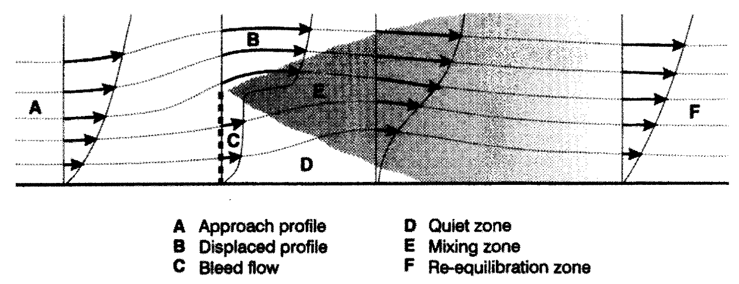
There is a specific effect due to the trunk of a tree: bottom gap (Mayaud, 2016]. The wind speed after the trunk will be higher than the wind speed before the tree, due to the compression caused by the crown (see here for an example).

Determining the Drag force coefficient through literature

On this web page the Drag force and Pressure-difference convention are built around:

• Δp: pressure difference
  So Δp is over the full length L.
• Derivative of Δp is dΔp/dx: pressure gradient
  Here dΔp/dx can change (which most of the time is assumed to be constant) over L. On this website this is not writen as Δp/Δx, but as dΔp/dx.
  
• F: drag force
  If there is an L on the right side of Δp formula: F = Δp*A
  In the case we have the area A on the right side of F formula and no L on the right side of dΔp/dx formula: F = (dΔp/dx)*A
  In most case A is assumed to be constant over L.

In Hagen (1971, formula [2]): D_h = F = ρ/2*u²*H*C_{dhag
<H is the height of the windbreak>}
With dΔp/dx =D_h/A → assume A=H²*π/4 → dΔp/dx = ρ/2*u²*[C_dhag/(H*π/4)]
C_d = C_dhag/(H*π/4)
Hagen (1971) gives an idea of C_dhag for an slatted fence (H_windbreak = 2.44m) with 40% porosity (and u's between 5.5 and 11m/sec): C_dhag = 1.17
C_d = 0.61

In Bitog (2012, formula (1)): Δp = m*ρ*u²*C_{dbit
<m is the thichness of the tree crown, aka L>}
dΔp/dx = ρ/2*u²*[2*C_dbit]
C_d = 2*C_dbit
Bitog (2012) gives an idea of C_dbit for an oak (H_tree = 5.5m): C_dbit= 0.55
C_d = 1.1

In Roubos (2014, formula under Fig. 127) : Q_w;rep = F = ρ*u²*A*C_{wrou
<A is the area of the tree crown>}
With dΔp/dx =Q_w;rep/A → dΔp/dx = ρ/2*u²*[2*C_wrou]
C_d = 2*C_wrou
Roubos (2014) gives an idea of C_wrou for an oak (H_tree = 15m): C_wrou= 0.25
C_d = 0.5

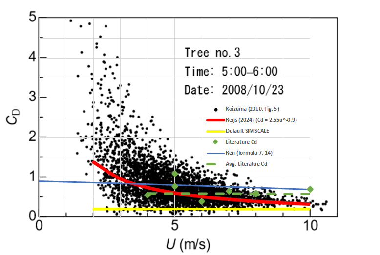
In Koizuma (2010, forumula1) : P_w = F = ρ/2*u²*A*C_{dkoi
<A is the area of the tree crown>}
With dΔp/dx =P_w/A → dΔp/dx = ρ/2*u²*[C_dkoi]
C_d = C_dkoi
Koizuma (2010) gives an idea of C_dkoi for poplar (H_tree = 12.5m):

• For leafless trees the C_dkoi is around 0.2 (Koizuma, 2010, Fig. 7) for u's between 4 and 11/sec.
• A leafed poplar has a C_dkoi (Koizuma, 2010, Fig. 6) between 0.55 (u = 4m/sec) and 0.3 (u = 11m/sec).
  

C_d = 0.55

In Ha (2018, page 24): P_w = F = ρ/2*u²*A*[C_dha]
_{<A is the area of the tree crown>}
With dΔp/dx =P_w/A → dΔp/dx = ρ/2*u²*[C_dha]
C_d=C_dha
Ha (2018, page 23) provides an average C_dha of 0.169 for u's between 2 and 10m/sec and leafless deciduous trees (average H_tree=17m).
Ha (2018, page 23) provides an average C_dha of 0.655 for u's between 4 and 10m/sec and leafed deciduous trees (average H_tree=17m).
C_{d = 0.655}

In Wikipedia:  C_dwiki is given for several objects
Wikipedia (Figure 2021, accessed Febr. 2024) has a C_dwiki of around 0.59 for an eliptical sphere (at Reynold number between 10⁴ and 10⁶).
C_d = 0.59

<sub>In Bekkers (2022, forumula1) : D = F = ρ/2*u²*A*Cdbek
<A is the area of the tree crown>
With dΔp/dx =D/A → dΔp/dx = ρ/2*u²*[Cdbek]
Cd = Cdbek
Bekkers (2022, Fig. 9) has a Cdbek of around 0.77 (at u = 5m/sec and Htree=6.5m).
Cd = 0.77

In Mayhead [1973] the Cd of several forest trees have been determined (Koizuma, 2010, Fig. 6].</sub>


In SIMSCALE (2023, Table 4)
SIMSCALE uses a C_dsim = 0.2 (regardless of the u, H or leaves).
C_d = 0.2

In Ren (2023, formula 4): S_i = dΔp/dx = -ρ/2*|u|*u*[C_dren]
C_d = C_dren
Ren (2023, page 7) has a C_dren of around 0.704 (at u = 10m/sec and H_tree=6.8m).
C_d= 0.704

Overview of found Drag force coefficients

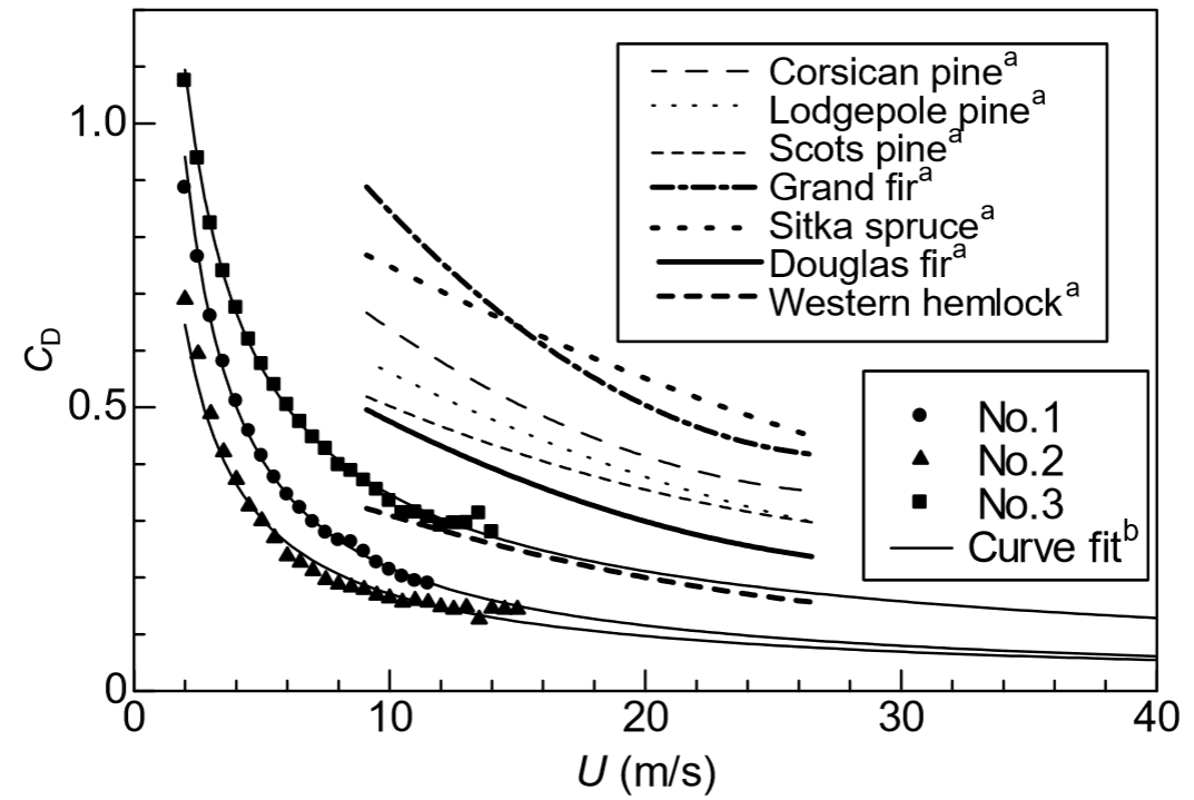
The above values of C_d (green is what the given values for leafed deciduous trees are in the reference) are put in below table:

It is assumed the crown height (H_crown) is 0.67*H_tree.
For determination f, the formula of SIMSCALE has been used.

Leaf Area Index

Some general aspects of C_d

The C_d is depending on:

• C_d is dimensionless [-].
  
• Difference between true area (the area of visible branches and leafs) and enclosed area (the area of the crown as whole) (Bekkers, 2022, page 3). Enclosed is being used on this web page.
• The C_d can be when the tree is a static/rigid object or dynamic when the tree form changes due to the wind velocity (Ren, 2023; Bekkers, 2022). Static is being used on this web page.

• The wind velocity is important for the value of C_d. The below picture is from Koizuma [2010, Fig. 5] (black dots), Reijs (red), Ren [2023, Formula 7 and 14] (blue curve) and SIMSCALE [2023)] (yellow curve):
  
  <3.4m/sec::3.0 Bauufort and 10.8m/sec:: 6.0 Beaufort>
  The red curve is C_d=2.55*u^-0.9 and thus an E=-0.9, which is close to the expected E value (~-1) for deciuous trees (Vogel, 1984, Table 1).
  The green dots are the C_d found in literature and SIMSCALE's C_dSIM=0.2 is the yellow line.
  These C_d don't seem to have a dependency on u (on average 0.6 [-] for the range 3 to and including 5Bft: dashed green line).
• The size of the tree also determines the C_d: the larger the tree the larger the C_d (Bekkers, 2022, page 9).
  

Forchheimer coefficient in SIMSCALE

In SIMSCALE (2022 and 2023): S = -ρ/2*|u|*u*f = -ρ/2*|u|*u*[2*LAD*C_dsim]
f_sim = 2*LAD*C_dsim = 2*LAI/H_crown*C_{dsim (see also in this SIMSCALE spreadsheet for this formula; tab Tree Model)}
<H is height of crown [H_crown=0.67*H_tree]; LAI is Leaf Area Index, C_dsim = 0.2>

Remark: C_d is depending on the velocity, so why is SIMSCALE's f_sim independing on velocity?
The following points are perhaps important to understand f_sim :

• When measuring the drag in e.g. a windtunnel: C_d is depending on wind velocity and on the leaf coverage (LAI) of the tree [Koizuma, 2010, Fig. 5]
• A leafless tree has a C_d=0.18 (migth be quite velocity indepepdent). And a leafed tree has an average C_d between 0.2 and 1.5 depending on wind velocity [Koizuma, 2010, Fig. 5]
  
• SIMSCALE uses: f_sim = 2*LAI/H_crown*C_dsim
• C_dsim =0.2 is independant on leaf coverage (LAI) and independing on wind velocity.
  
• So questions:
• What is C_dSIM scientific bakground? At what velocity and what leaf coverage?
  
• How would one simulate a tree: a) a porous cylinder of crown height and raised with stem height, b) a porous cylinder of tree height (not raised) or c) a solid thin stem and a porous cylinder of crown height? Proposed to use a) (and alternatively c).
  

Valideren van CAD-model van een boom

Periode voor bebladerd en kale bomen verkregen via Temple (pers. comm. 2024)

Bebladerde boom (voor mei t/m september)

Kale boom (voor november t/m maart)

Determining the Forchheimer coefficient through simulated emperical way

It is assumed that for the Darcy-Forchheimer metholdogy only the Forchheimer coefficient is important when dealing with trees, see also here (section Tree Model).

First simulation iteration

• a blobbed object with openings between the blobs to proxy porosity, so no porocity medium is needed and
• a stacked-cylinder object which will need a porous medium definition

stacked-cylinder objects:

From this analysis it is clear that a leafed tree (using

Second simulation iteration

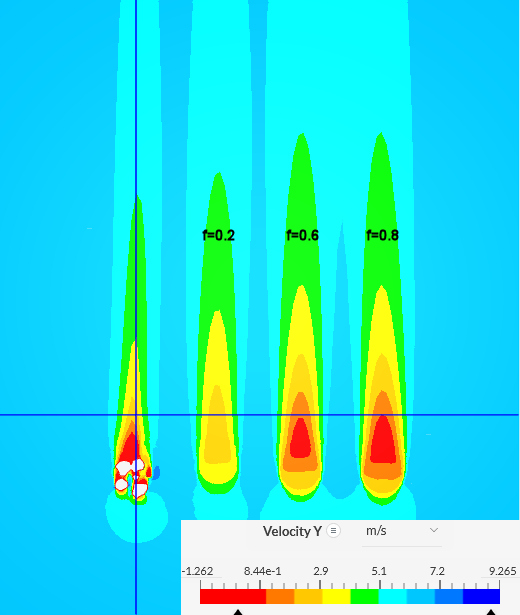
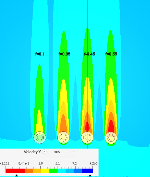
Here is an analysis done for f = 0.1 (leafless tree), 0.35 (like close to SIMSCALE), 0.45 and 0.55 (so only stacked-cylinder objects):

Proposed to do a third iteration with; f = 0.09 (leafless tree), 0.375, 0.4 and 0.425

Third simulation iteration

Here is an analysis done for f = 0.9, 0.375, 0.4 and 0.425:

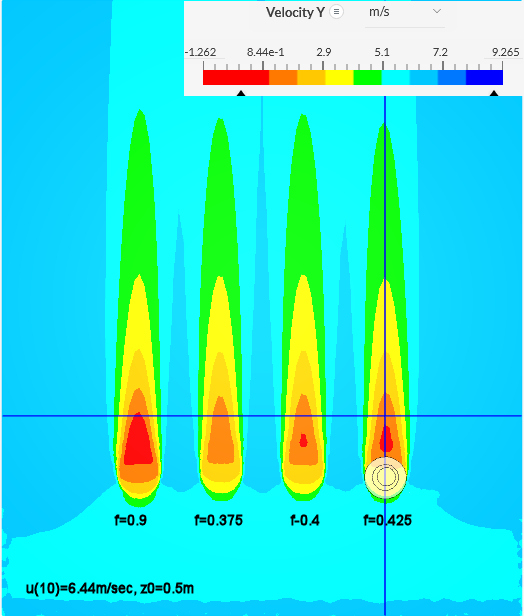
So f=0.425 looks to be ok-ish for a leafed tree (@ u(10)=6.44msec and z₀=0.5m).

Fourth simulation iteration

Here is an analysis done for f = 0.09 (leafless tree), 0.4, 0.425 and 0.45:

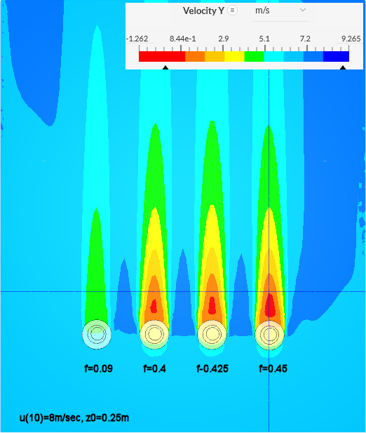
So the leafed tree with f=0.45 looks best @ u(10)=7.17m/sec (u(H_tree)=8m/sec) and z₀=0.25m.

Compare stacked-cylinder tree with real tree

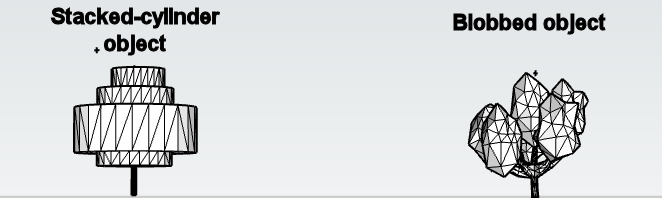
The CFD behavior (H_tree=15.5m, H_crown=11.5m, z₀=0.25m, u(H_tree)=8m/sec) of the stacked-cylinder object with Darcy-Forchheimer medium or the blobbed object without Darcy-Forchheimer medium, provides a good match with the velocity distribution of the real leafed tree (Ren, 2023, Fig. 16a2):

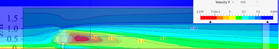
In above graph the bottom gap due to the tree truk is seen: the light-blue patch [due bottom gap] below the red patch [mixing zone].

Using f_VR = 2*LAI/H_crown*C_dSIMVR, would make a C_dSIMVR of 0.65 (= f_VR*H_crown/2/LAI = 0.45*11.5/2/4).

Proposed Forchheimer coefficient for a tree with other H_othertree, H_othercrown, LAI_other and u_other

Derived reference parameters (from above comparison) are:

f_ref ~ 0.45 [1/m] at H_reftree=15.5m, H_refcrown=11.5m, LAI_ref=4 and u_ref(H_reftree)=8m/sec

For other H, LAI and u:
f_other = f_ref * H_refcrown / LAI_ref * LAI_other  / H_{othercrown =} 1.29 * u_comp * LAI_other  / H_othercrown

with:
u_comp=( u_other(H_othertree) / u_ref(H_reftree) )^0.3 (using emperical optimisation) -> 0.52 * u_other(H_othertree)^0.31

Porosity and Forchheimer coefficient relation through simulated emperical way

Be sure to check if porosity is optical or aerodynamic. As optical is easier to measure (take a photo), this has been utilised on this page. The conversion can be seen here [Gonsales, 2018, Figure 9]:
AP = OP^0.65

Below formula need to be checked (as the AP formule was wrongly transcribed and also the exponene has been changed, from 0.65 (Gonsales, 2018, Figure 9) or 0.36 (Grant&Nickling, 1998; Ren, 2023]

An optical porosity = -0.267*LN(f)+0.1267 formula was derived by matching the results of Darcy Forchheimer coefficent (f) and Perforated plate (Free area ratio=optical p[orosity]) simulations of a stacked-cylinder object in SIMSCALE (honeypot):

The optical porosity [Gonsales, 2018, Figure 9] formula = -0.267*LN(f)-0.0108 is also derived from above picture:

Reijs (2024, f - blue), Hagen (1971, C_d - grey), Stichlmair (2010, C_d - formula (11) and (13); thick plates are assumed to have relatively small holes: yellow), SIMSCALE (f - green) are different, but perhaps not that far off.
Hagen and Stichlmair don't work with trees, but fences or plates.

Conclusions

Referenties

Acknowledgements

Disclaimer and Copyright
HomeUpSearchMail