 Home
Home Up
Up Search
 Mail
Mail NEW
40m NVIS experiences by Victor Reijs
is licensed under CC BY-NC-SA 4.0


Checked SDRs between 28/8/2026 15:15UTC and 7/9/2026 15:20UTC:
| Location (link) |
Distance from Lemelerveld [km] |
Proxi. |
Avg. Elev [deg] |
Azi [deg] |
Comment |
| IJsselmuiden | 30 |
Nearby |
88 |
296 |
down from 6/9/2026 21:15 UTC |
| UTwente |
43 |
Nearby |
87 |
121 |
|
| Dokkum |
101 |
Nearby |
82 |
347 | working again from 29/8/2026 16:50UTC |
| Maasbree |
125 |
Nearby |
80 |
189 |
|
| Fordham |
430 |
Far |
60 |
270 |
Lost many measurements, as session times out after 60min/day. Down between 5/9/2026 10:20UTC and 6/9/2026 12:25UTC |
Click below graph to get the latest version
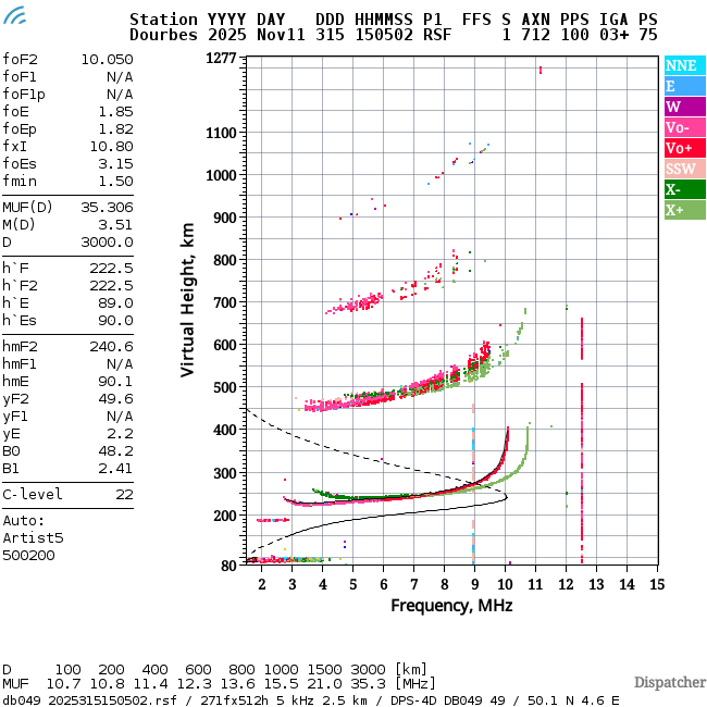
of the ionogram at Dourbes (Belgium).
Archives for the ionograms are here
(click for URSI: DB049, select Year, Month
and Day, and select the Measurement Time)
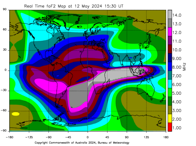
Here is an Earth ionogram map (from The
Bureau of Meteorology) of the foF2 values; a pity there is
no such map for fxI (one can approximate fxI by adding some 0.74MHz to foF2 (Male [2021] mentions
0.7MHz):
Each measurement session contained 17 data points:
The TX was made ready by:
 |
 |
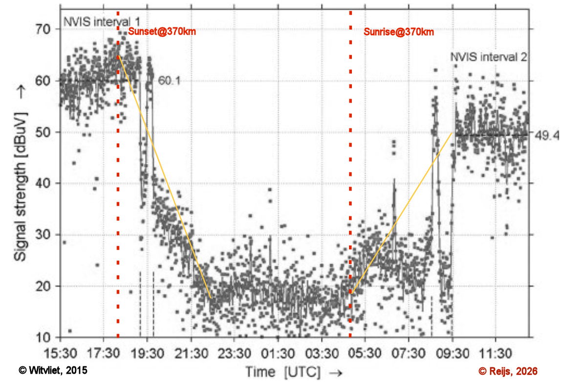
| Signal strength (SS)
[Witvliet, 2015,Fig 23] |
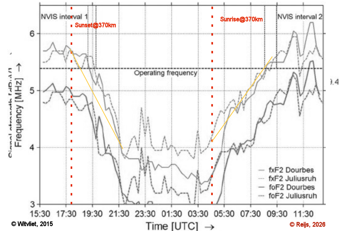
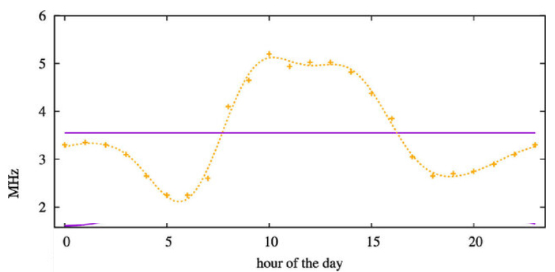
fxI and foF2 [Witvliet, 2015,Fig 24] |
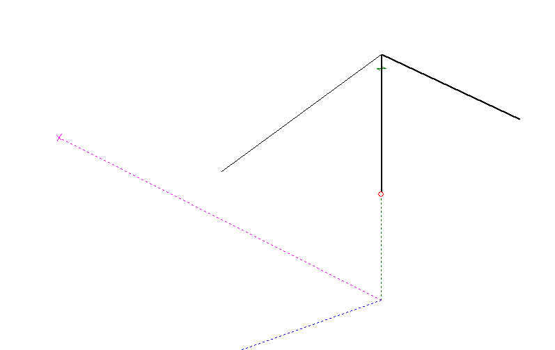
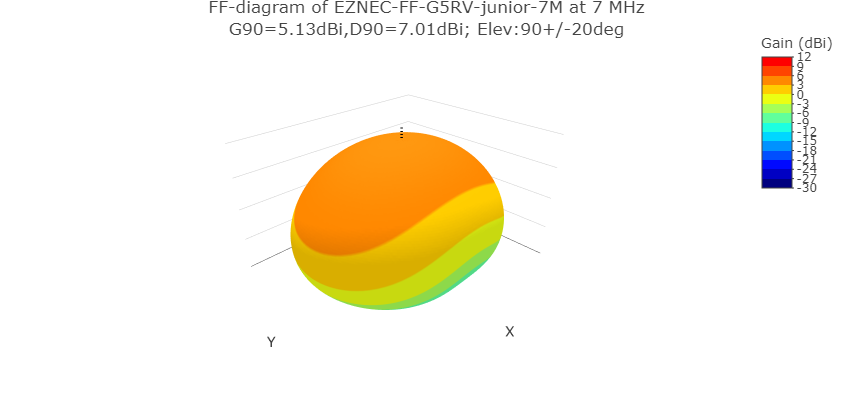
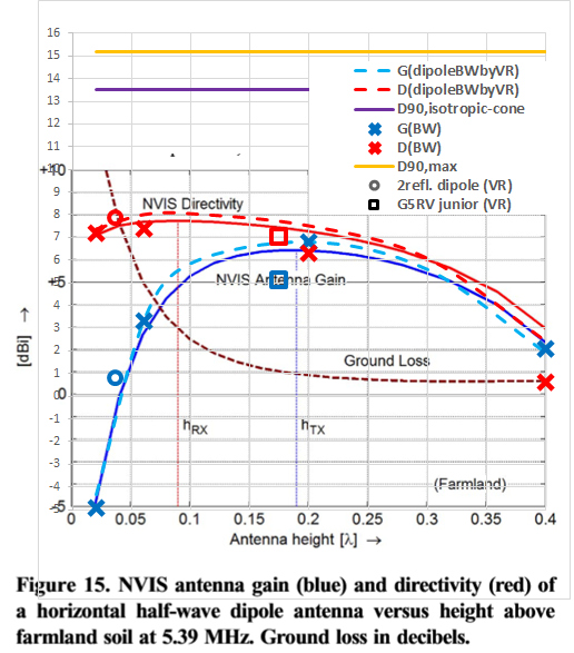
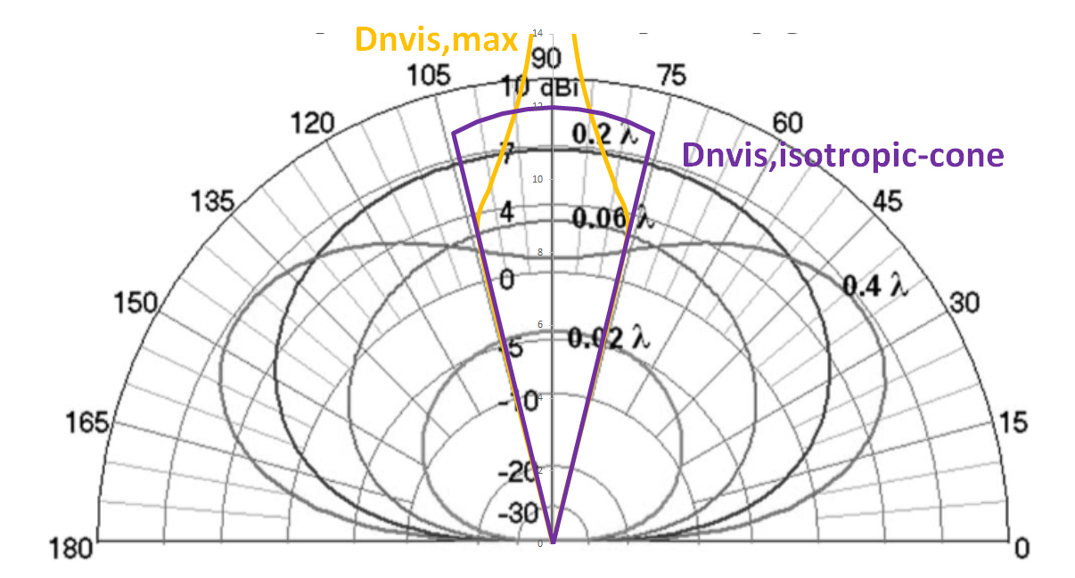
Average height of G5RV junior as inverted V is around 7m (aka
0.175λ). The centre was at 9.3m and the ends are at 5m and 7m.
QTH PE1ATN: border of Lemelerveld.
| 40m |
20m |
10m |
|
| G90 [dBi] | 5.13 |
0.28 |
0.92 |
| D90 [dBi] | 7.03 |
1.67 |
2.75 |
| G20 [dBi] | -2.43 |
1.05 |
1.8 |
| D20 [dBi] | -0.53 |
2.45 |
3.63 |
| Elevation step [deg] |
Difference [dB] |
| 10 |
0.8 |
| 5 |
0.4 |
| 2.5 |
0.2 |
| 1 |
0.1 |
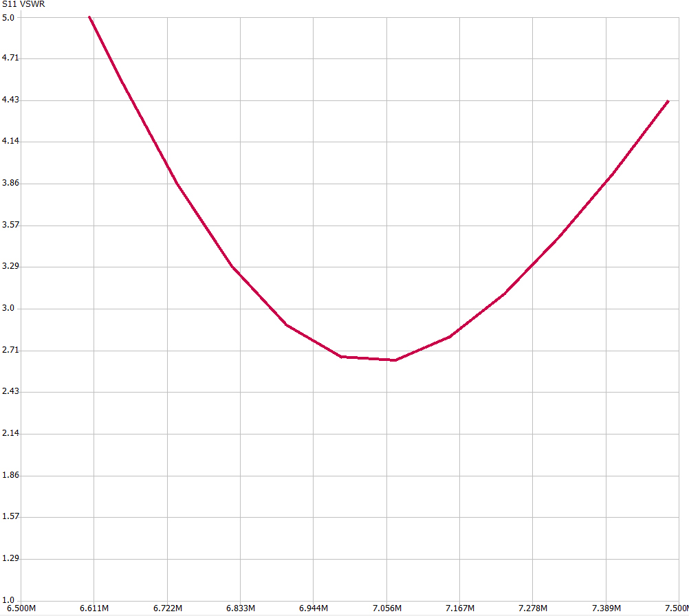
| NanoVNA |
EZNEC Pro2+ urban |
|||
| Band |
fr |
SWR |
frs | SWRs |
| 40m |
7.0 |
2.7 |
6 |
4.6 |
| 20m |
15.0 |
1.3 |
15.6 |
1.6 |
| 10m |
28.5 |
1.3 |
27.7 |
1.1 |
From 8/9/2026 to 9/9/2026 measurements were done every 5minutes to see why there are these fluctuations sometimes seen.
See for the actual measurement sessions see this pageDate from 28/8/2026 until 2/9/2026:
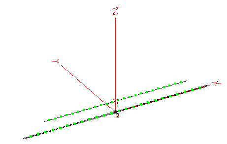
The design of this dipole came from here. Height of 40m dipole is around
1.45m (aka 0.035λ) and has two reflectors wires at ground level.
QTH PE1ATN/P: beside Overijssels kanaal near Lemelerveld
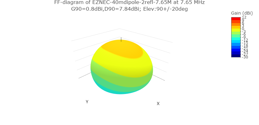 .
.
| 40m |
15m* |
|
| G90 [dBi] | 0.8 |
1.17 |
| D90 [dBi] | 7.87 |
5.38 |
| G20 [dBi] | -7.91 |
-2.34 |
| D20 [dBi] | -0.85 |
1.85 |
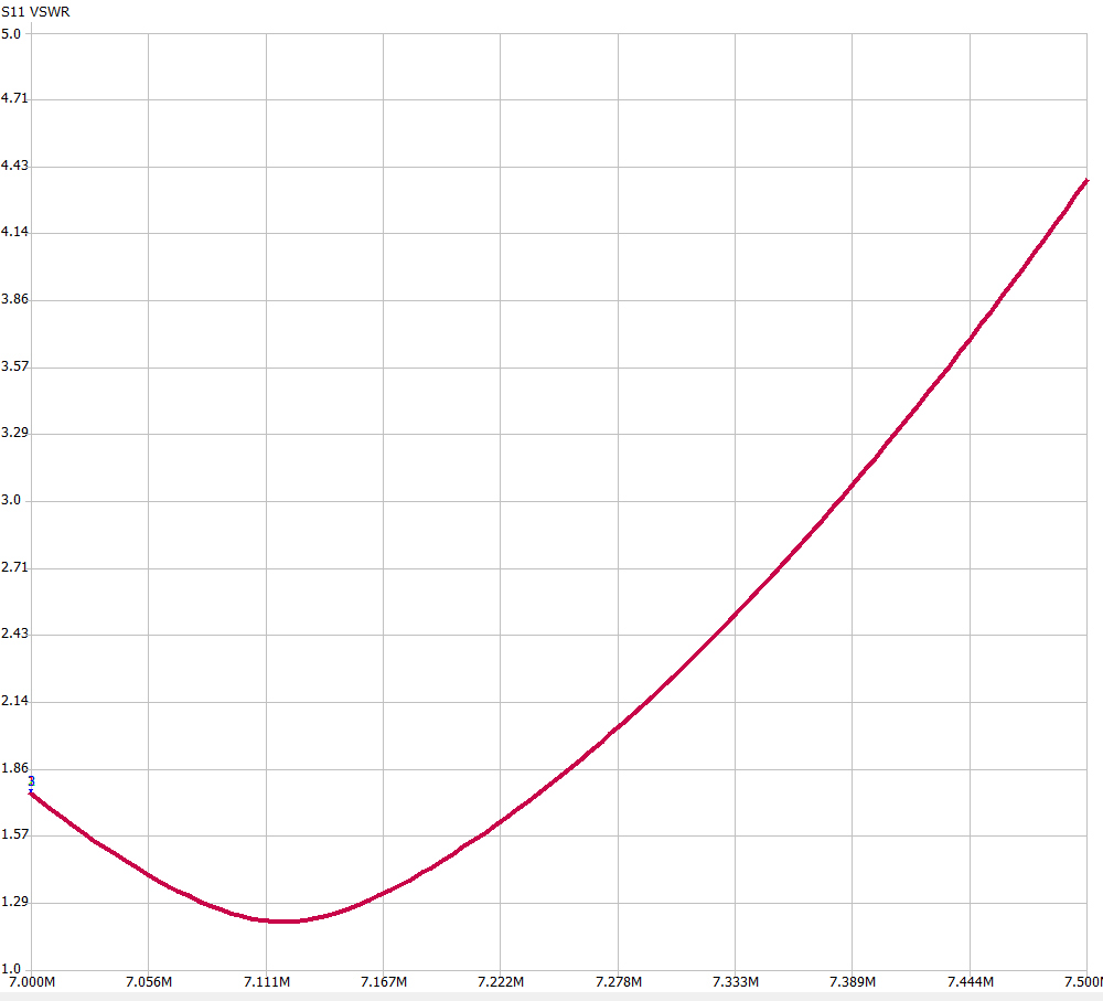
| NanoVNA |
EZNEC Pro2+ farmland |
|||
| Band |
fr | SWR |
frs | SWRs |
| 40m |
7.04 |
1.2 |
7.66 |
1.8 |
See for the actual measurement sessions (up to now only 1) this page.
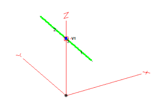
Average height of G5RV as dipole is around 20m (aka 0.25λ).
QTH PE1ATN/P: at Scouting Lemelerveld.
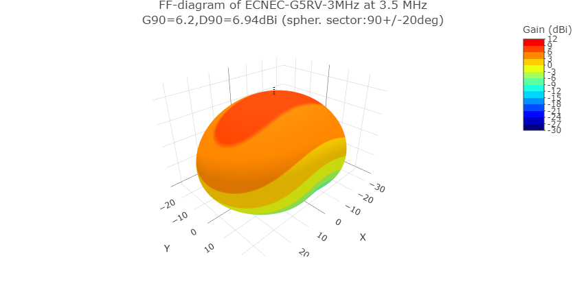
| 80m |
¬40m |
20m |
15m |
¬10m |
|
| G90 [dBi] | 6.2 |
-0.28 |
-5.77 |
-2.44 |
1.24 |
| D90 [dBi] | 6.94 |
0.68 |
-4.75 |
-1.51 |
2.24 |
| G20 [dBi] | -0.93 |
3.05 |
2.17 |
1.97 |
2.77 |
| D20 [dBi] | -0.2 |
4.01 |
3.18 |
2.89 |
3.77 |
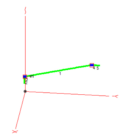
The lowest (start) point of EFHW is around 5m and the heighest
(end) around 10m.
QTH PE1ATN: border of Lemelerveld.
 |
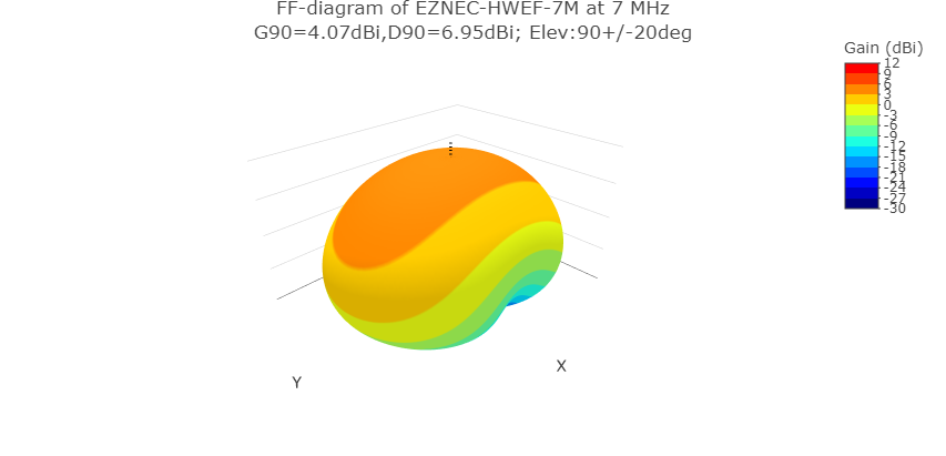 |
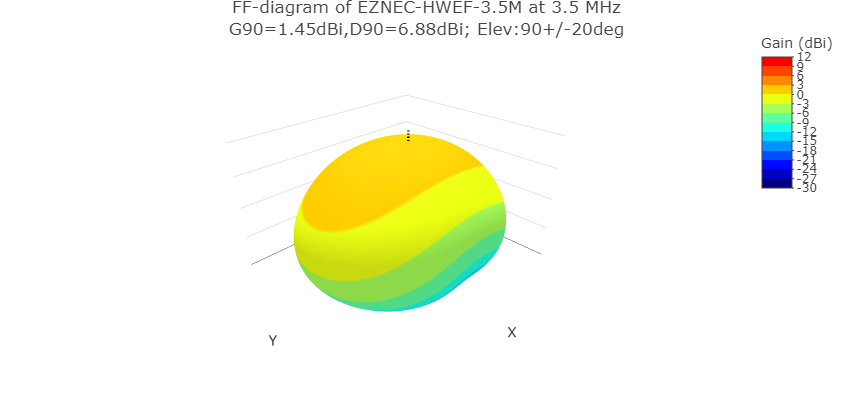
So the EFHW has NVIS properties around 3.5 and 7MHz (simulated in EZNEC Pro2+ v.7.0; using NEC-2, elevation angle step=1deg).
Using Witvliet, formula (2) and (3) [2015], we get (elevation angle step=10deg):
| 80m |
40m |
20m |
15m |
10m |
|
| G90 [dBi] | 0.76 |
4.09 |
-1.26 |
-1.14 |
-3.75 |
| D90 [dBi] | 6.99 |
6.98 |
0.89 |
0.83 |
-1.95 |
| G20 [dBi] | -7.74 |
-3.67 |
0.43 |
1.43 |
2.21 |
| D20 [dBi] | -1.51 |
-0.78 |
2.59 |
3.41 |
4.01 |
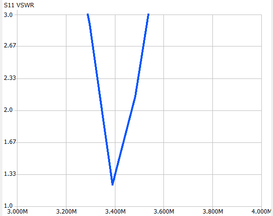
| NanoVNA |
EZNEC Pro2+ farmland |
|||
| Band |
fr | SWR |
frs | SWRs |
| 80m |
3.39 |
1.2 |
3.5 |
1.5 |
| 40m |
||||
| 20m |
||||
| 15m |
||||
| 10m |
||||
The SWRs values look ok-ish.
The frs is around +4% different for 80m.
<is being measured>
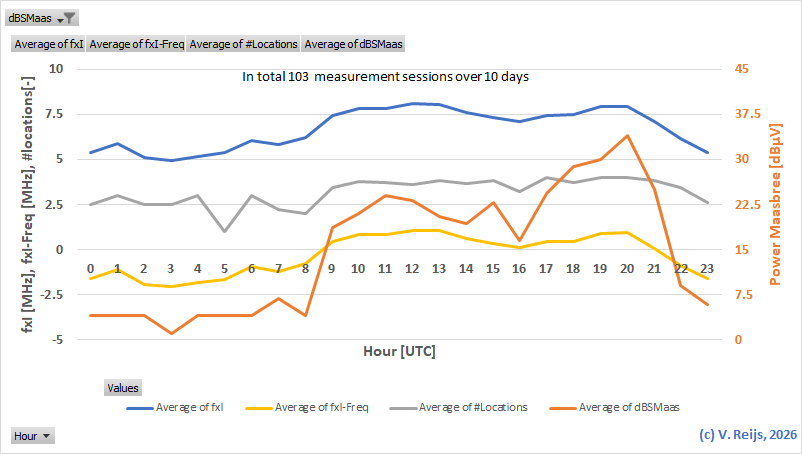
It looks that fxI is a better threshold value for possible
communication than foF2. As soon as fxI drops below TX Freq., the
propagation does down with some 25dB (from measurements of Reijs).
Similar can be seen in Witvliet [2015, Fig.23 and 24]. The average
height of the fxI layer is around 340km.
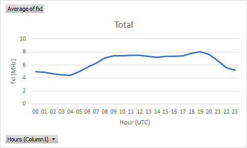
The fxI is on average 0.74MHz higher than
foF2.
The elevation is never very close to 90deg, as the underlaying layers (like E and F1) will have already refracted the wave front; so the wave front will not reach F2 at 90deg, but a few degrees less [Witvliet, 2015, section 3.1].
After Sunise/set (at the location of the F-layer) one can see a
slow change of the fxI and RX signal strength.
The signal strength in Witvliet and Reijs are similar when
including the extra TX of 22dB in Witfield; and both see a signal
range-variation of some 15dB.
Both Witvliet en Reijs see that the signal strength in the evening
is larger than in the morning: Witvliet some 11dB (Witvliet, 2015,
Fig. 23] and Reijs some 8dB.
There is still propagation even when the fxI is much lower than
the test frequency (like fxI-Freq = -2MHz). The night time
signal strength of Witvliet is around 18dBμV (@850W) and for Reijs
this is around 5dBμV (@5.5W). When including the TX strength
diffence this becomes: 18dBμV (Witvliet) and 27dBμV (Reijs).
All waves transmitted during night time will be in
some way scatter down and up and this will cause night-time
scatter. This night-time scatter signal is much weaker than
normal daytime NVIS: often 45 to 50 dB down from a true reflected.
In the cause of Reijs and Witvliet the difference is respectivily
some 25 and 35dB.
The dip in signal
strength looks to be related to the fxI dip around noontime. The
reason is the so-called noontime-bite-out (typically forced by
thermospheric winds).The closer the fxI is to the TX Freq,
the larger the signal strength dip looks to be.
The increase of the signal strength looks to happen around the
Sunrise at 340km (location of the height of fxI layer). The
decrease of the signal strength looks to happen around the Sunset
at 340km (location of the height of fxI layer.
The duration of these increase and decrease are different
(primarily due to a more rapid buildup of solar ultraviolet
radiation in the morning) for Witvliet and Reijs (also
knowing the difference in measurement accuracy (Witvliet Minutes;
Reijs in Hours):
| Measurement |
Month |
Increase duration [hours] |
Decrease
duration [hours] |
| Witvliet |
November |
5 |
3.5 |
| Reijs |
September |
6 |
3 |
It could be that fluctuations cause
temporarily increase of signal strength (if fxI is close to TX
Freq; at the time 17:25 on 8/9/2026 it shows clearly).
A similar effect (except the geometry [aka non-NVIS] is different)
might have been seen with the frequency deviations in the Doppler
measurements.
Witvliet [2015, Section 5.3] also sees such fluctuations of the fxI value: his
'hesitations'.
Some measurements:
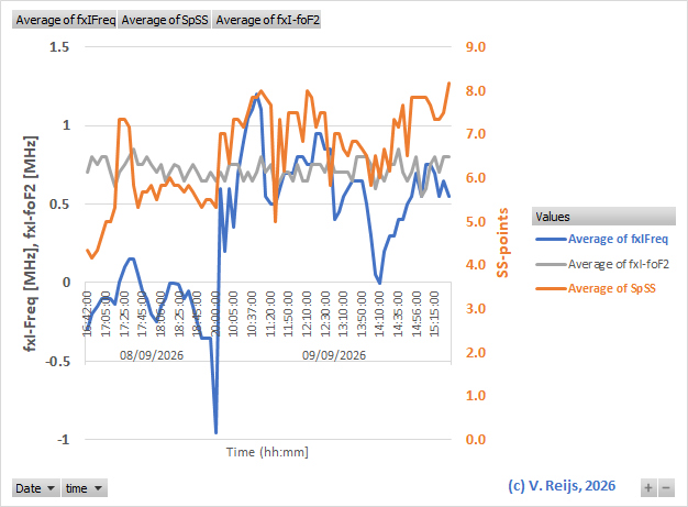
The Time axis looks continuous, but there are
gaps in data points!
Of the simulated 40m antennas (NVIS dipole, G5RV and EFHW); my
G5RV junior looks to be the most effective (highest G90
and D90), followed by EFHW and then the NVIS dipole.
EZNEC Pro2+ uses NEC-2 as the underlaying calculating engine. The
ground-modelling is Sommerfeld-Norton.
The difference between Witvliet simulation [2015, Fig. 15] using
NEC-4 and Reijs' simulation using NEC-2 is
quite small (less than on average 0.2dB).
Would be interesting to see a better simulation for the frs
when uisng NEC4 or NEC-5, as it can deviate some + or -10% at frequencies of 7MHz
when using NEC-2. If someone wants to help me running that,
please let me
know.
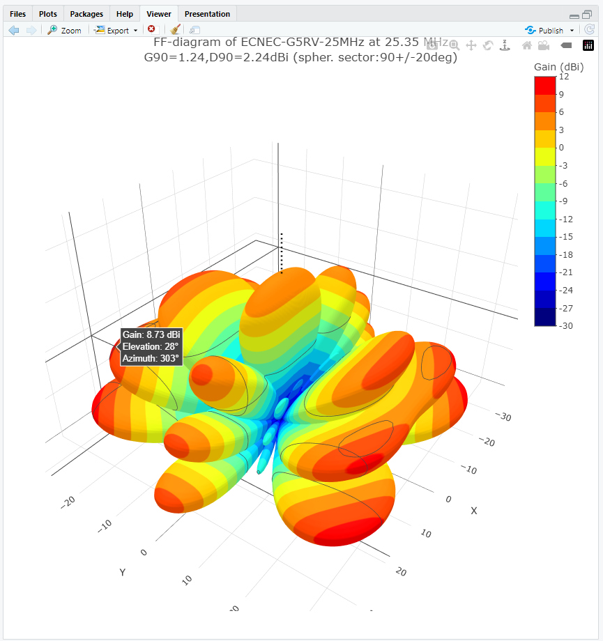
In Excel a spreadsheet has been made which can receive the
FF-diagram data and calculate the G90 en D90.
Based on that experience, a extended version has been made (with
help of Google AI, although a lot of understanding and debugging
is still needed!) with R that can: import EZNEC 3D FF data; import
manual FF-diagram data; convert 3D FF-diagrams into an
onmnidirectional FF-diagram; configurable elevation direction
(elevation agle xx) and cone size (practicality of this still
needs to be investigated); calculate Gxx en Dxx;
and plot FF-diagrams with the calcuated info:
Chen, Yiding et al.: Latitudinal dependence of daytime electron
density bite-out in the ionospheric F2-layer. In: JCR space
physics (2020), issue 10.1029/2020JA028277, pp. 1-12.
Male, Jordi et al.: Analysis
of the ordinary and extraordinary ionospheric modes for NVIS
digital communications channels. In: Sensors 21
(2021), issue 2210.
Poole, Ian: Radio progation: Principles & practice. Herts,
RSGB 2007.
Sapundjiev, Danislav and Stanimir Stankvc: Statistical analysis and modeling of the local
ionospheric critical frequency: A mid-latitude single-station
model for use in forecasting. In: Acta Geophysica 64
(2016) issue 3, pp. 810-824.
Walden, M.C.: The extraordinary wave mode: Neglected in
current practical literature for HF NVIS communications. In:
Ionospheric radio Systems and Techniques.2009.
Witvliet, Ben A. et al.: Near vertical incidence skywave propagation:
elevation angles and optimum antenna height for horizontal
dipole antennas. In: IEEE Antennas and Propagation Magazine,
57 (2015), issue 1, pp. 1-18.