HomeUpSearchMail
NEW

CFD meshing tests

CFD meshing tests by Victor Reijs is licensed under CC BY-NC-SA 4.0

Introduction

Looking at a cubic of 10x10x10m (P(10)), tests have been held with increasing the number of mesh cells (aka decreasing the mesh-grid size).

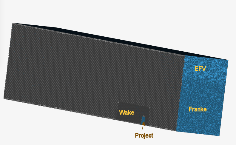
So the simulation is about a cube (10x10x1m) and it has four mesh areas:

1. around the cube: mesh P(roject)
2. An area around the wake: mesh W(ake)
3. An areas that is close to Franke's advice for the size of a wind tunnel: mesh F(ranke)
4. The EFV (External Flow Volume) size, slightly higher than Franke: mesh E(FV)

Below is a view (through the middle of the cube) of these four mesh areas:

Convergence study

In this study the 1D-size has been changed with a factor of 1.26 (see proposed by SimScale); meaning the 3D-volume changes with a factor of 2 .

Convergence

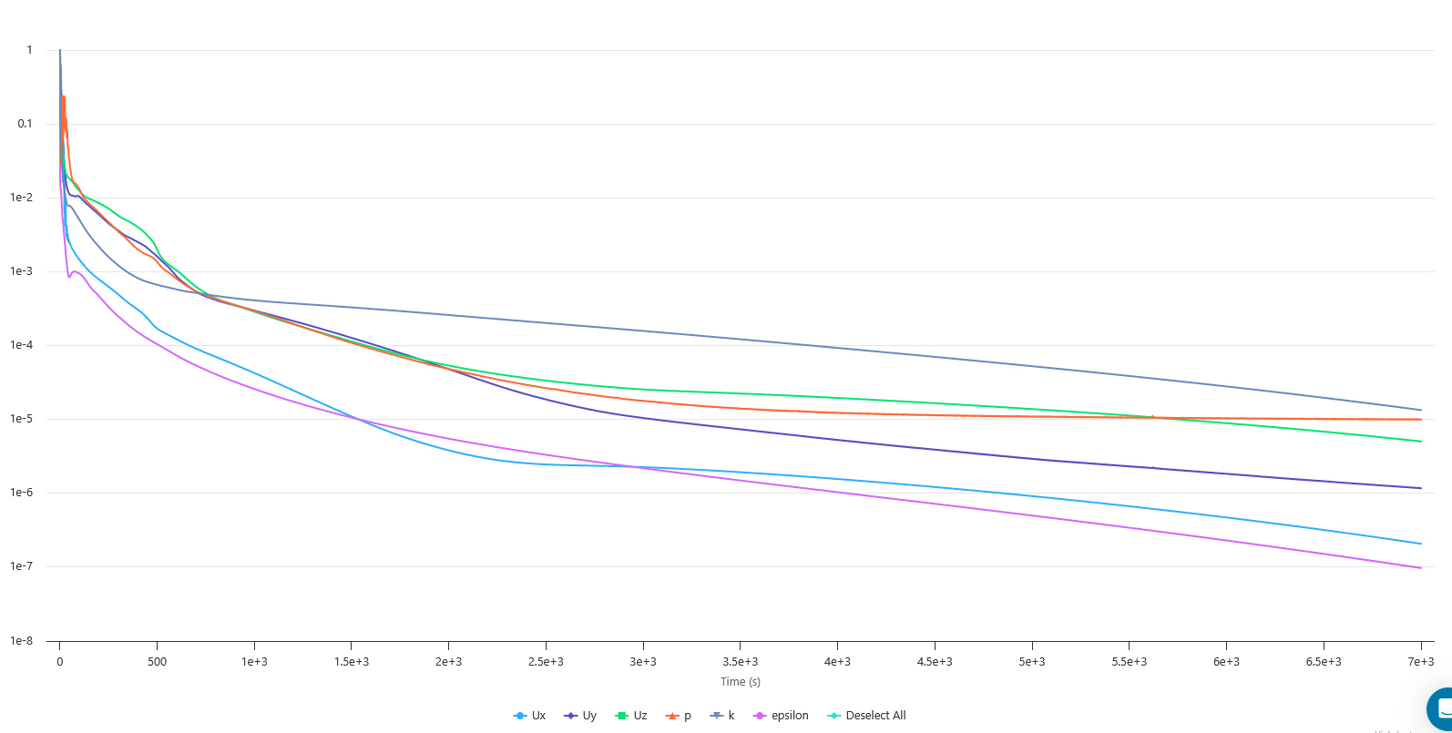
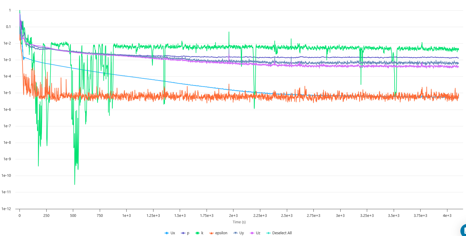
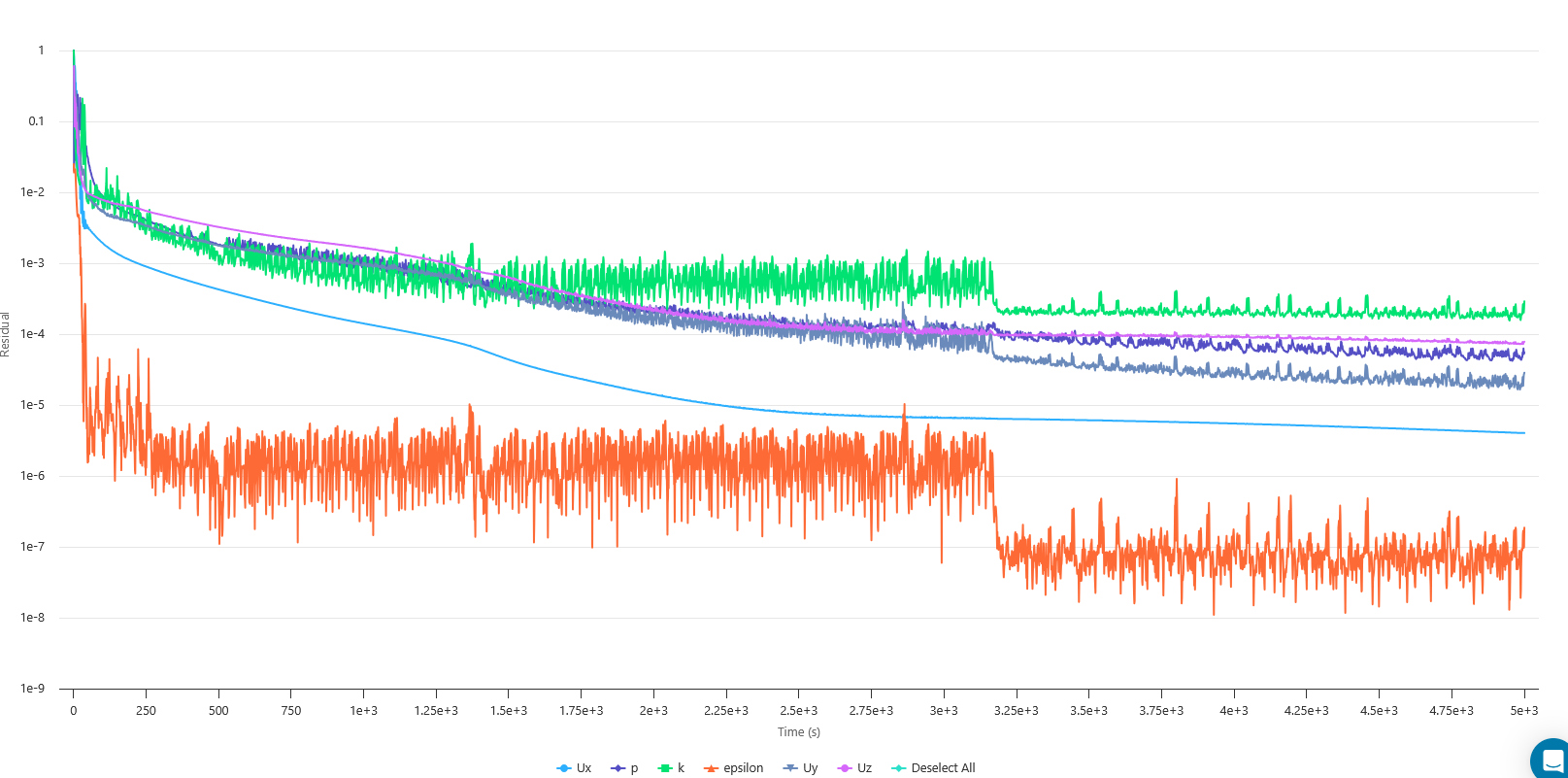
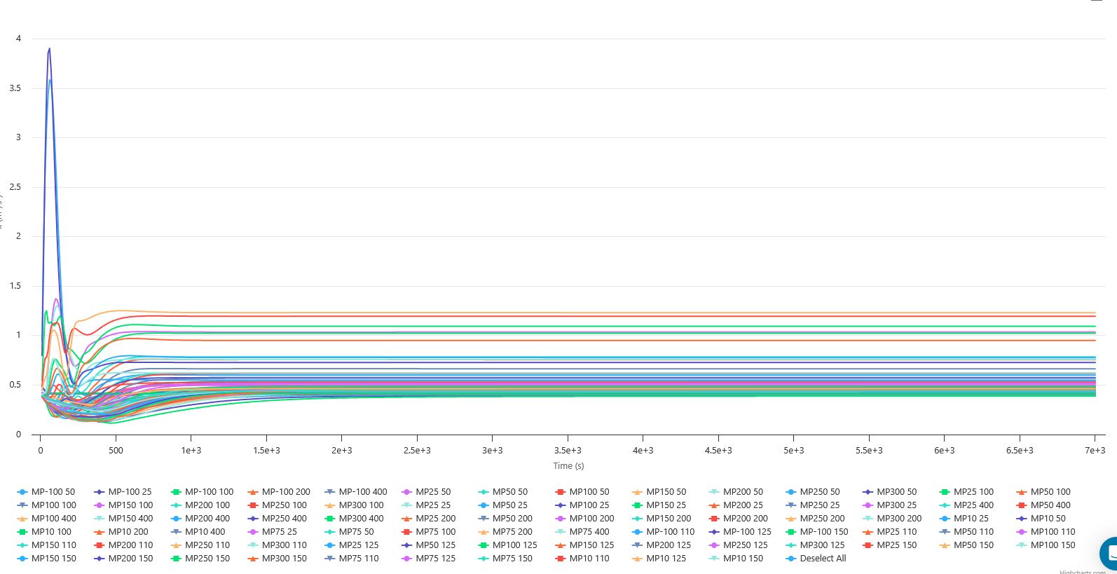
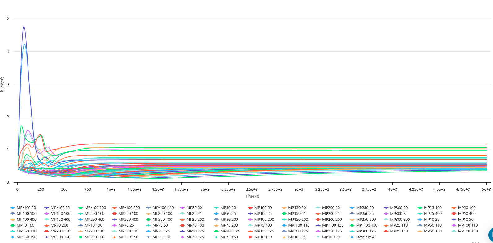
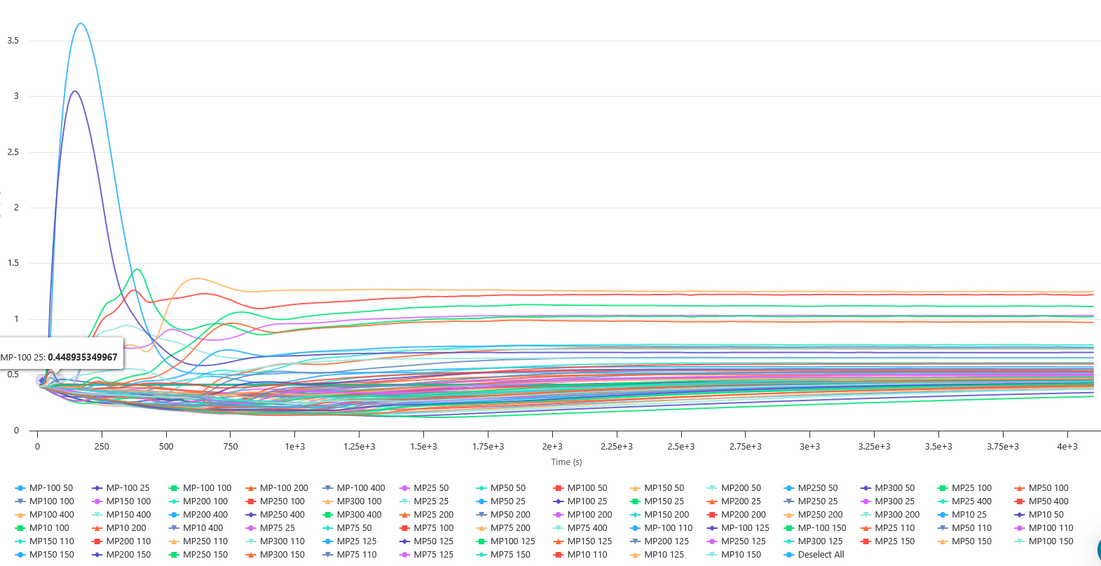
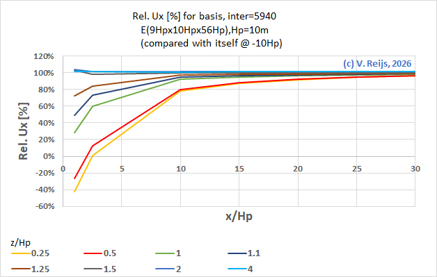
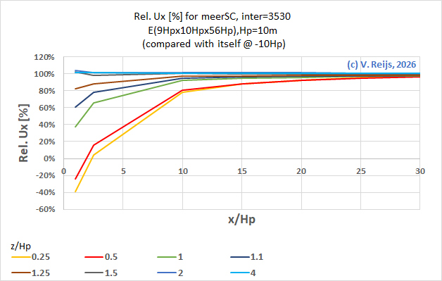
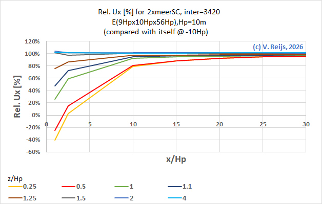
Mesh-size	Convergence Plot - Residual	Probe point convergence	Relative Ux (SF) depending on x/Hp (parameter z/Hp)
default
meer
2xmeer

One can see oscillatory convergence of the residuals, but no (observable) oscillation in the probe points values.

Oscillatory convergence

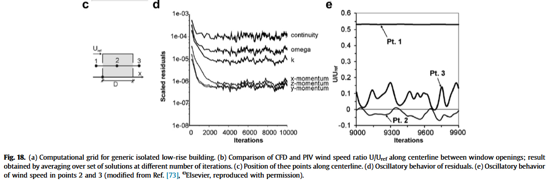
From Brocken [2015, Section 5.6]:

In addition to these valuable guidelines, the present paper warns for oscillatory convergence in steady RANS simulations. When flow problems that are inherently transient are forced into a steady simulation, and when numerical diffusion is limited, it is possible that oscillatory convergence occurs. This implies that not a single converged solution is obtained, but that the solution depends on the number of preceding iterations [73]. This is not an indication of a lower-quality simulation. On the contrary, it indicates that the grid resolution is high enough and numerical diffusion is low enough for non-linear effects to influence the convergence process. A detailed comparison by Ramponi and Blocken [73] of such CFD results with the high-quality Particle Image Velocimetry (PIV) measurements by Karava et al. [266] indicated that accurate results could only be obtained by averaging the CFD results over at least a period of oscillatory behavior. In addition, these simulations showed that the results at different numbers of preceding iterations corresponded to modes of the actual transient behavior of the natural ventilation flow, with a flapping jet entering the building and with signs of vortex shedding in the wake. Fig. 18 illustrates some results of this study. Fig. 18c-e shows the oscillatory behavior of the converged solution, where oscillations are found for all residuals (Fig. 18d) but not for all points in the flow field (Fig. 18e). Note that points 2 and 3, which show oscillatory convergence, belong to the regions in the actual flow field that are characterized by unsteadiness (flapping of jet in pt 2 and vortex shedding in pt 3).
The advice is to first allow convergence to continue until residuals do not change any more or enter into oscillatory convergence. In the latter case, the iterative process should be continued and solutions at different stages in this second part of the iterative process should be stored and averaged to yield the final averaged solution.

Influnce of #mesh-cells on relative speed (SF)

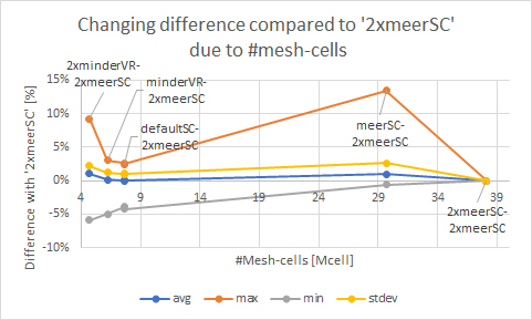
Comparing the Rel. U_x (Speed Factor SF) of the different #mesh-cells with the Rel. U_x of #mesh-cells 2xmeer or default, we get the following graph:
<by the way; averaging of the U_x [as proposed in Karava, reference by Brocken, had no significant influence on this comparison>

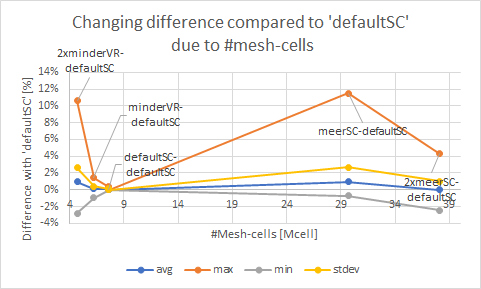The form of the two graphs is similar; except the difference is zero [of course] for the #mesh-cells compare with.

One would though expect an increasing difference between decreasing #mesh-cells. This is not happening for '2xmeer' and 'meer'.

Question: Why is this? What is now the best number of mesh-cells?

References

Blocken, Bert: Computational Fluid Dynamics for urban physics: Importance, scales, possibilities, limitations and ten tips and tricks towards accurate and reliable simulations. In: Building and Environment 91  (2015), pp. 219-245.

Acknowledgements

Disclaimer and Copyright
HomeUpSearchMail