NEW
This web page will look into measurements of coils, chokes and transformers in the range of 1 to 50Mhz (covering the ITU definition of MF and HF ranges from 300kHz to 30MHz). The following sections are covered:
The aim of this web page is to determine which Hybrid
Choke/Transformer to use for a 40m OCFD. The compenents making up
the Hybrid are also individually measured, using different devices
and different metholdogies. Also the properties of the OCFD are
measured and compared with other people's measurements and
literature. A conclusion will be provide where the synthesis of
these compents is discussed (to provide a design and
implementation template).
Work in progress: Hopefully I will gain more knowledge to use
proper naming.
Choke and Transformer look
to have clear meaning/function to me and I think these can cover
some/all of the bullets (as an added property) in the Balanced and
Unbalanced section.
I will use the word balun on this webpage only to pointout a physical device. How the device is configured/used, determines if it is a Choke or Transformer. Additional input and output properties are added to define if the configuration is Balanced/Symmetrical or Unbalanced/Asymmetrical.
Proper naming is important, and it has to be consistent and
understood by me and others;-) To accomodate others, I have
included in the below sections alternative terms used by others.
Anyway this web page should be build in such a way, that if a name
changes it will be simply changing strings of letters.
Several (closely related) directions are refered to, when using
the terms Balanced (bal) and Unbalanced (un):
It is sometimes not clear what is meant with the terms Balanced
and Unbalanced, so asking/digesting the meaning is important. The
last bullets sounds the most clear...
One can have un-un, bal-un and bal-bal.
IEV definition: Balun:
device for transforming a balanced voltage to an unbalanced voltage or vice-versa.
I am still strungling with the term balun in many publications.
For now: I don't look at this abbreviation of BALanced/UNbalanced,
but see it as a string of five letters (aka an icon).
On this web page, a balun (not using a capital...) is defined as a
4 port device (2 input and 2 output ports). It is constructed with
2 or more tightly coupled coils. The coils (twisted pairs, mono,
bifilar or twin, coax, stripline, etc.) can have different layouts
(toroid, tube, λ/4 or λ/2, etc., around/inside a material) and
core material (air, iron, NiZn, MnZn, dielectric, etc.). The
interconnection/configurations of the coils determines its
function, resulting in a Choke or Transformer.
According to W7EL (page
159): A voltage balun causes equal an opposite voltages
[defined from Earth] to appear at the balanced port regardless of
load impedances
According to W7EL (page 159): A current balun causes equal an opposite currents to appear at the balanced port regardless of load impedances
IEV definition: Choke:
an impedance transforming device for
preventing energy within a given frequency band from taking an
undesired path.
Other terminology: 1:1 balun, current balun, common mode choke,
sheath current choke, Tranmission Line-Transformer (TLT).
The aim of a Choke is to make sure that on each of the two outputs
equal but opposing currents exist (there is no transforming
aspect, so always 1:1).
If the socalled 1:1 balun chokes the Common Mode Currents
(CMC), I call it on this webpage a Choke.
IEV definition: Transformer:
electric energy converter without moving
parts that changes voltages and currents associated with
electric energy without change of frequency.
Other terminology: x:1 balun, voltage balun,
voltage/impedance/current transformer, Tranmission
Line-Transformer (TLT), autotrafo.
The aim of a Transformer is to make sure that the voltage and thus
impedance/current is transformed: these three are of course
directly coupled through Ohm's law.
IEV definition: One-dimensionally
distributed two-terminal-pair circuit element characterized by
lineic inductance l, lineic capacitance c, lineic resistance r
and lineic conductance g which may all be functions of the same
space coordinate x, where the voltage u(x, t) and the electric
current i(x, t), where t is the time, are related by partial
differential equations
Other terminology: feed lines, feeders, coax, twin-pair
Can be balanced (twisted pair, twin-pair, bifilar) or unbalanced
(coax).
Assume a current in each of the two wires (resp. i1
and i2). Looking at the same point along their length,
one measures i1 and i2; the Differential
mode current in each wire is (i1 - i2)/2 and
the Common mode current in each wire is (i1 + i2)/2.
A 'nice' explanation of Common
mode current is in many case by done looking at Coax cable. Where
the in- and outside of the Coax braid are seen as two conductors.
The TEM mode can only exist between the inside of Coax braid and
the outside of the Coax inner conductor (the Differential mode
current). While the outside of the Coax braid can be 'utilised'
for something else (like Common mode current).
I have a few issues with this 'nice' explanation:
A more general
explanation of how common mode current works in all types of
cables could be the following:
At this moment the simple explanation of muRata works for me
best: part of the energy (current) goes through stray capacitances
from the antenna through the Earth or antenna feed to the earth of
the rig. Beside this, noise sources can also intorduce common mode
currents. These currents through Earth are resulting in a common
current in the cable (be it symmetric or asymmetric cable).
I am open to other
explanations.
The aim is to understand if theory and pactice match.
Only using one (composite) coil of the Chokes/Transformer (but not really checking
the full Choke/Transformer function, that is for a later section):
just to make some basic measurements of a coil's (mutual)
induction, capacitance, resistance. These basic measurements are
to to learn the test tools (Component tester and NanoVNA). The
measurements are using Reflection measurements.
| wire-s11s21-core |
Measured on wire |
Side/color |
Toroid core |
Part of Choke / Transformeree |
Windings through hole (N) |
Component tester |
NanoVNA (Reflection measurement at 10 kHz) |
Calculated ALct [µH/N2] |
Calculated ALNV [µH/N2] | Setup |
Link | NanoVNA (Saver) (Series-through measurement) |
|||||||||
| Lct
[µH] |
RDC
[Ω] |
Inter
coil Cw [pF] |
LNV
[µH] |
f1 when S11 Phase=0 [MHz] |
Intra
coil Ct [pF]a |
f2
when S21 Phase=0 [MHz] |
M [µH]b |
S21f1 [dB] |
Zf1 [Ω]c |
S21f2 [dB] |
Zf2 [Ω]c |
||||||||||
| rg58a-ss-43 | RG58A/Ue |
braidbraid |
FT140-43 | 1:1Guanella | 8 |
60 |
0.2 |
(34) |
56 |
0.94 |
0.88 |
9.28 |
2.46 |
31.28 |
59.29 |
-26.399 |
2000 |
-37.855 | 7700 |
||
| rg58a-ii-43 |
RG58A/Ue | inin |
FT140-43 |
1:1Guanella | 8 |
60 |
0 |
(34) |
~58 |
0.94 |
0.91 |
8.24 |
3.13 |
31.28 |
59.30 | -26.394 |
2017 |
-35.013 |
5532 |
||
| rg58a-is-43 | RG58A/Ue | inbraid |
FT140-43 | 1:1Guanella | 8 |
- |
- |
34 |
- |
not connected | 9.2 |
2.51 |
31.28 |
59.29 | |||||||
| rg316-ii-43 | RG316e | inin |
FT140-43 |
1:1Guanella | 14 |
280 |
0.3 |
(36.5) |
160 |
1.43 |
0.82 |
4.88 |
1.91 |
17.84 |
277.93 |
-33.335 |
4575 |
-39.738 |
9603 |
||
| rg316-ss-43 | RG316e | braidbraid | FT140-43 | 1:1Guanella | 14 |
290 |
0.2 |
(36.5) |
172 |
1.48 |
0.88 |
4.4 |
2.26 |
18.8 |
288.15 |
||||||
| rg316-is-43 | RG316e | inbraid | FT140-43 | 1:1Guanella | 14 |
- |
- |
36.5 |
- |
not connected | 5.36 |
1.55 |
19.28 |
283.21 |
|||||||
| bi-1w1w-61 | twistedd
PTFE |
1white1white | FT140-61 |
4:1Ruthroff |
16 |
40 |
0.2 |
(17.5) |
37 |
0.16 |
0.14 |
9.68 |
3.47 |
23.6 |
37.83 |
-29.30 |
2800 |
-58.39 |
83000 |
||
| bi-1r1r-61 | twisted PTFE | 1red1red | FT140-61 | 4:1Ruthroff | 16 |
40 |
0.2 |
(17.5) |
37 |
0.16 |
0.14 |
9.68 |
3.47 |
24.08 |
37.92 |
||||||
| bi-1r1w-61 | twisted PTFE | 1white1red |
FT140-61 | 4:1Ruthroff | 16 |
- |
- |
17.5 |
- |
not connected | 10.16 |
3.15 |
24.08 |
37.88 |
|||||||
| bi-2r2r-43 | bifilar PTFE | 2red2red |
FT140-43 | 1:1DG0SA |
11 |
120 |
0.1 |
(22.5) |
93 |
0.99 |
0.77 |
2r in parallel (L) |
https://www.electronics-tutorials.ws/inductor/parallel-inductors.html | 6.8 |
2.29 |
31.76 |
118.99 |
-30.741 |
3376 |
-39.9 |
9785 |
| bi-2w2w-43 |
bifilar PTFE | 2white2white |
FT140-43 | 1:1DG0SA | 11 |
120 |
0.1 |
22.5) |
101 |
0.99 |
0.83 |
2w in parallel (L) |
https://www.electronics-tutorials.ws/inductor/parallel-inductors.html | 6.8 |
2.29 |
34.16 |
119.12 |
||||
| bi-2w2r-43 |
bifilar PTFE | 2red2white |
FT140-43 | 1:1DG0SA | 11 |
- |
- |
22.5 |
- |
not connected | 7.28 |
2.00 |
37.52 |
119.27 |
|||||||
| bi-1r1r-43 |
bifilar PTFE | 1red1red |
FT140-43 | 4:1Sevickf | 11 |
120 |
0.1 |
??? |
0.99 |
7.76 |
- |
7.76 |
- |
||||||||
| bi-1w2w-43 | bifilar PTFE | 2white1white |
FT140-43 | 4:1Sevickf | 11*3 |
3290 |
0.3 |
??? |
960 |
3.02 |
0.88 |
in plus series (3L+6M=9L) |
22.64 |
- |
22.64 |
- |
|||||
| bi-2w2w-43 | bifilar PTFE | 2white2white |
FT140-43 | 4:1Sevickf | 11 |
130 |
0.1 |
??? |
1.07 |
7.52 |
- |
7.52 | - |
||||||||
| bi-1r2r-43 | bifilar PTFE | 2red1red |
FT140-43 | 4:1Sevickf | 11*3 |
3350 |
0.3 |
??? |
1000 |
3.08 |
0.92 |
in plus series (3L+6M=9L) |
22.64 |
- |
22.64 |
- |
|||||
| bi-1w2r-43 |
bifilar PTFE | 2red1white |
FT140-43 | 4:1Sevickf | 11*4 |
crash |
0.3 |
??? |
??? |
n/a |
??? |
in plus series (4L+8M=12L)??? |
|||||||||
| bi-1w1w-43-01 |
monofilair PTFE |
1white1white |
FT140-43 | 1:1DG0SA | 11 |
110 |
0 |
(7.5) |
0.91 |
??? |
6.8 |
2.51 |
31.76 |
107.49 |
-30.338 |
6580 |
-39.19 |
18220 |
|||
| bi-1w1w-43-02 | monofilar PTFE |
1white1white | FT140-43 | 1:1DG0SA | 11 |
110 |
0.1 |
(7.5) |
0.91 |
6.32 | 2.41 |
31.76 | 107.59 |
||||||||
| bi-1w-1w-43 | monofilar PTFE |
1white-1white | FT140-43 | 1:1DG0SA | 11 |
- |
- |
7.5 |
- |
not connected and different coil |
8.72 |
2.47 |
33.68 |
107.53 |
|||||||
| bi-1was1w-43 | monofilar PTFE |
1white+1white | FT140-43 | 1:1DG0SA | 11*2 |
0 |
0 |
??? |
2 |
- |
in anti series (2L-2M=0L) |
https://www.electronics-tutorials.ws/inductor/series-inductors.html | - |
- |
- |
- |
|||||
| bi-1wps1w-43 | monofilar PTFE |
1white+1white | FT140-43 | 1:1DG0SA | 11*2 |
760 |
0.1 |
??? |
447 |
0.79 |
0.92 |
in plus series (2L+2M=4L) |
https://www.electronics-tutorials.ws/inductor/series-inductors.html |
2.48 |
- |
5.36 |
- |
||||
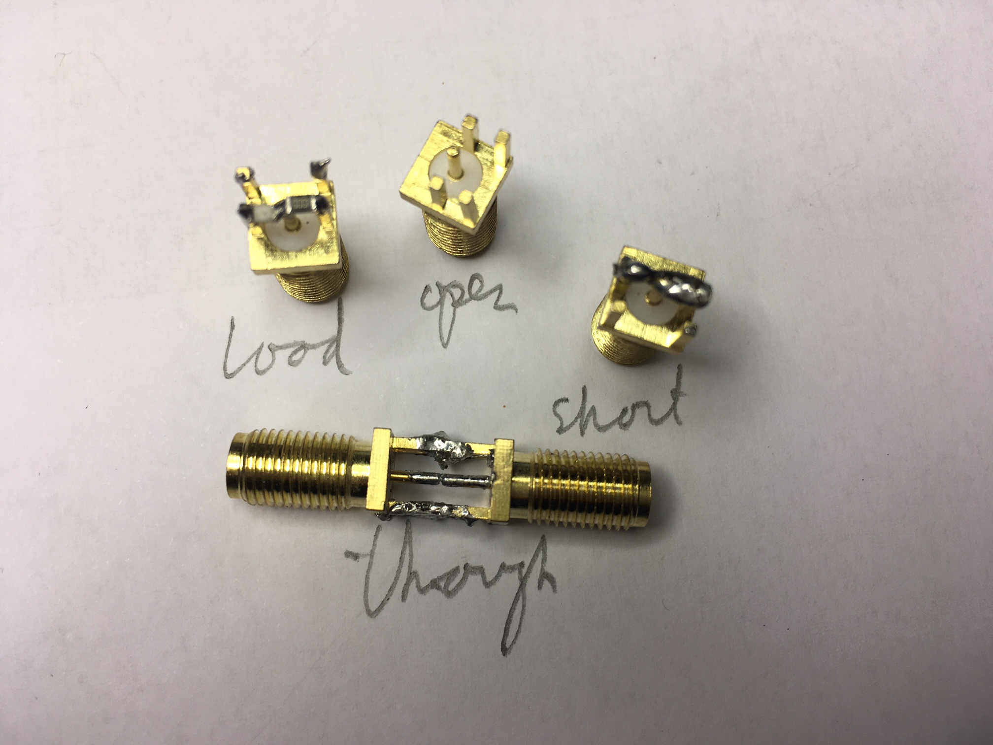
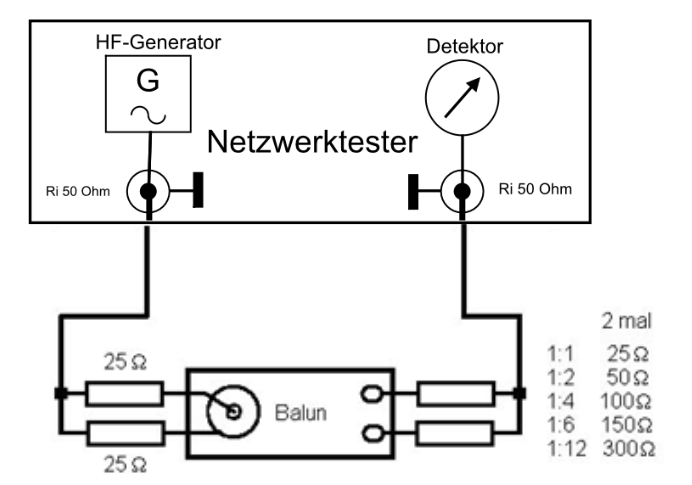
It is important to calibrate my NanoVNA
(one direction two ports calibration) using the SOL
(Short-Open-Load) method (for Reflection [somethimes called Shunt]
measurements) or the SOLTI (Short-Open-Load-Through-Isolation)
method (for Series-through and Shunt-through measurements);
The SOLTI devices used are seen in below picture:
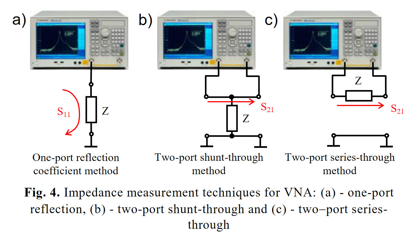
The three different setups can be used for three different ranges of
impedance (see alos this link, page 10):
In some cases one needs to include a connector setup which are
not easy to include in above calibration (also called de-embedding the
connectors).
For this web page the NanoVNA numbers have not been
de-embedded. Another alternative (in case the extension is
behaving as a 50Ω transmission line) is using the Calibrate
-> Offset delay feature on NanoVNA Saver or Display
-> Scale -> Electrical delay on the NanoVNA.
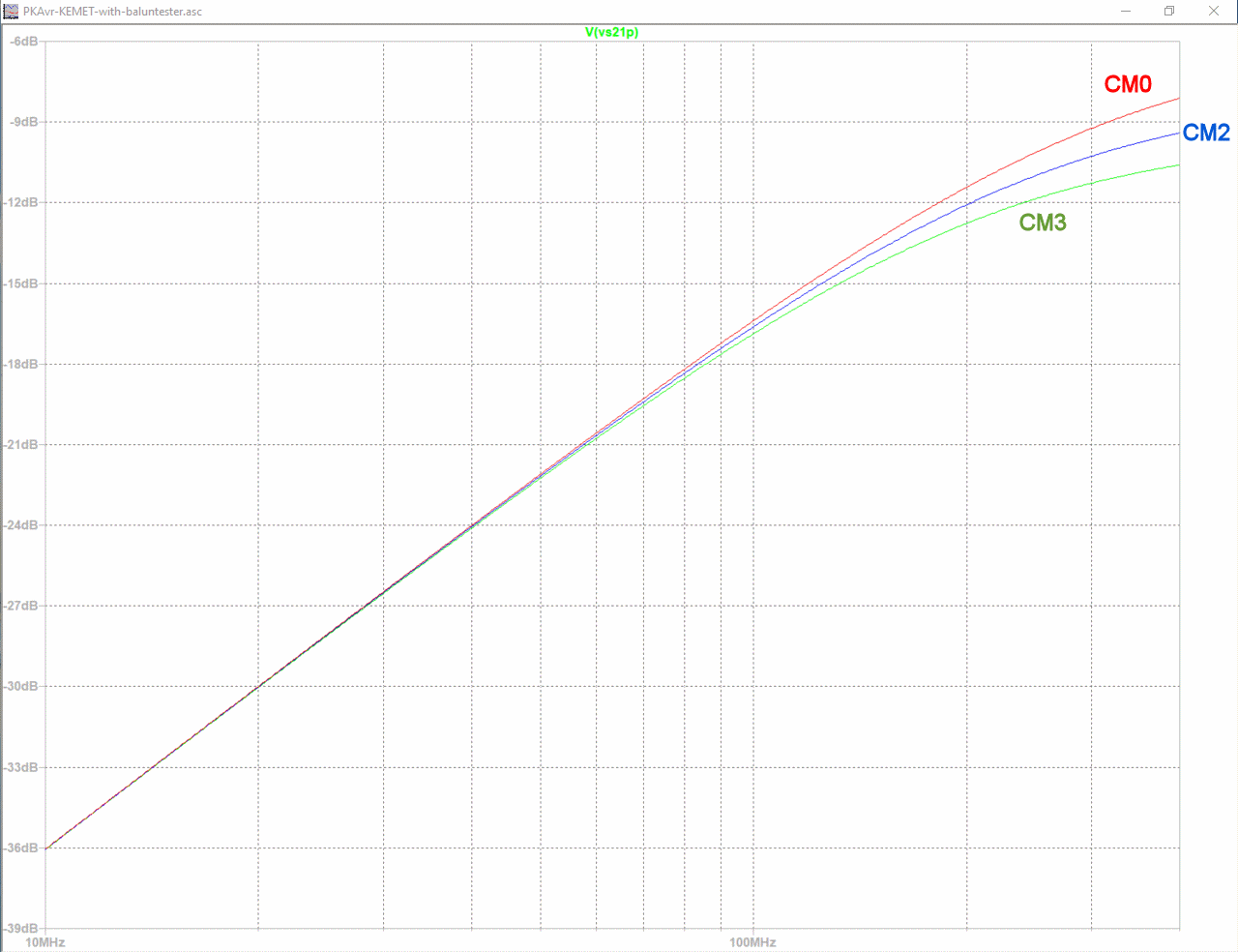
There is no real difference between these three CM-variants (see
below simulation in LTspice): upto 400MHz there is only 3dB
difference in S21 between CM3 and CM0, and below 100Mhz
there is no significant different.
When we are looking a Transformers and Chokes, f1 and f2
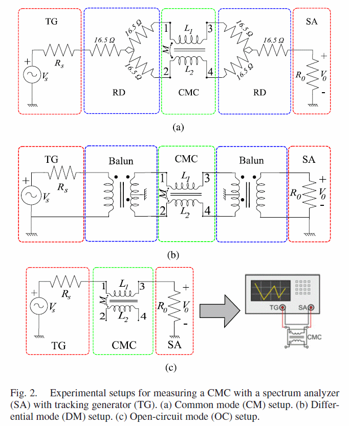
become fOC1 and fOC2 for the OC mode.
In most cases Zf1
and Zf2 will be Zcm and Zdm.
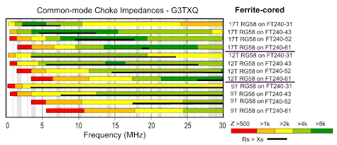
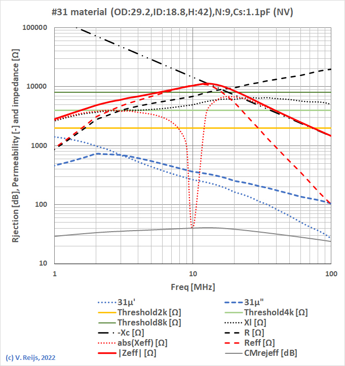
I think G3TXQ uses OC measurements. He
warns that the reactance of a Choke should be at least more than
several positive kΩs (to overcome the negative reactance of the
antenna feeder, which is several negative 100Ωs). But it is anyway
important to have a large resistance for a Choke. This garantees
that the |Z| is high (several kΩs).
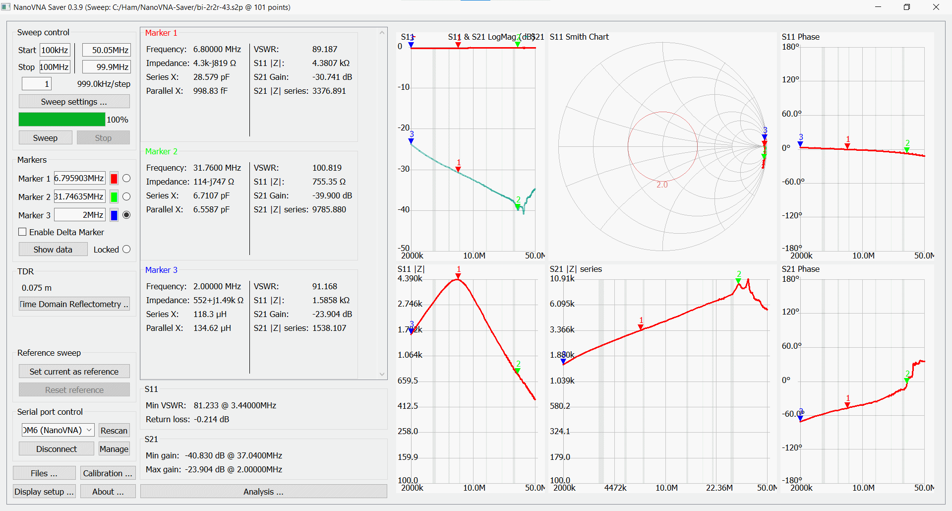
To see if a simulation is close to the Series-through (in this
case also OC mode) measurements, bi-2r2r-43 (bifilar PFTE coil with 10
windings) has been used.
As the Series-through measurements is also an OC mode test: Zf[1,2]
become R[cm,dm].
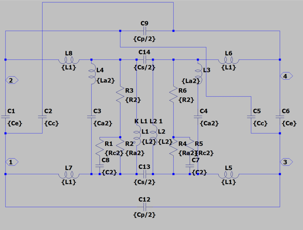
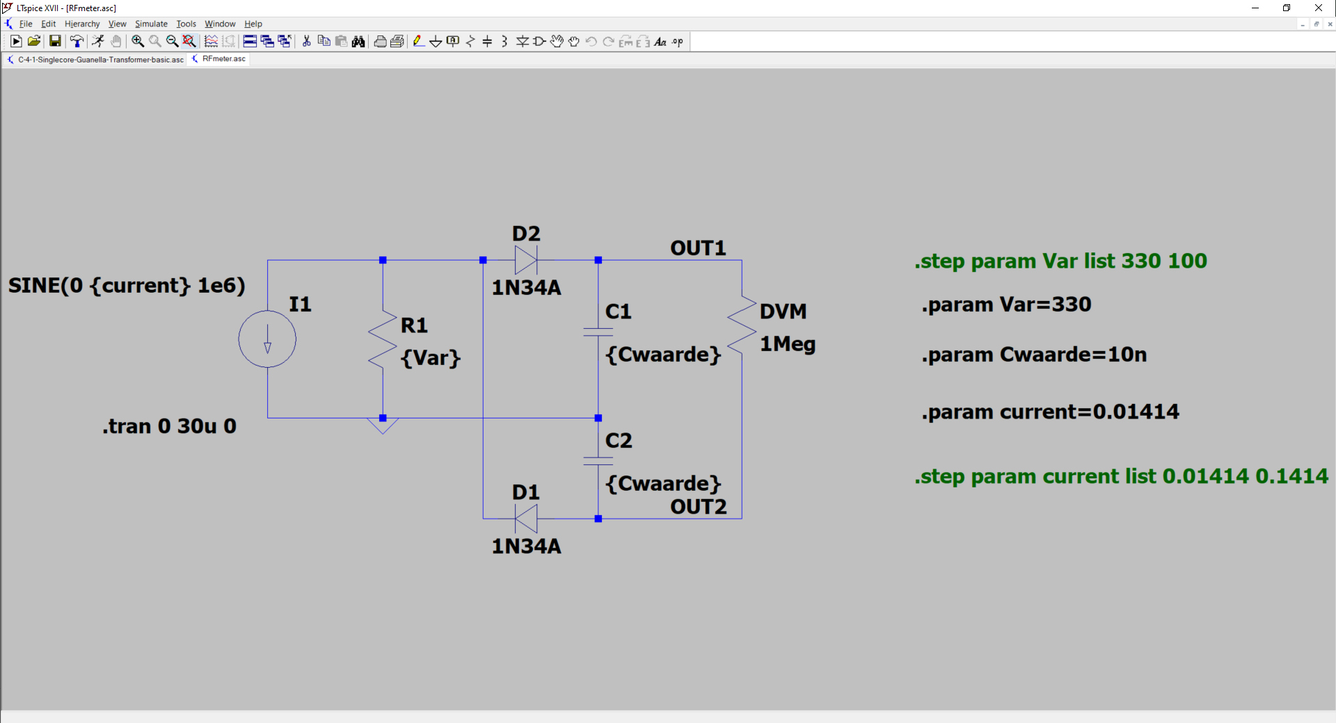
Two different type of equivalent circuit models have been worked
out: power-supply
choke (two monofilar multi layer coils) and MF and HF choke
(transmission line: one bifilar/coax single layer coil).
The Series-through measurements using NanoVNA Saver gives (power,
impedance and frequency axes are logarithmic, phase axis is
liniair):
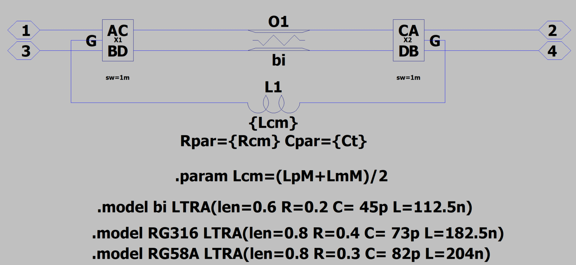
All circuit are based around RLGC models.
The equivalent circuit (for simulation
in LTspice and from the reference discussed here) of a
power-supply choke is below (send me an e-mail if you want the LTspice model
files):
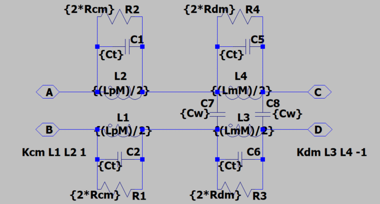
<The above circuit has been changed somewhat from the original article: RCM and RDM (capital letter subscripts) have been replaced by 2*Rcm and 2*Rdm (small letter subscripts) to match the above definition of Rcm and Rdm>
Using this power-supply equivalent circuit in LTspice XVII and
the parameters measured of power-supply chokes in the above
article (Tabel III), one can fully reconstructed the paper's
results over the frequency range of 0.1 and 10MHz.
And the simulation results (from LTspice) are (power, impedance and frequency axes is logarithmic and phase axis are liniair):
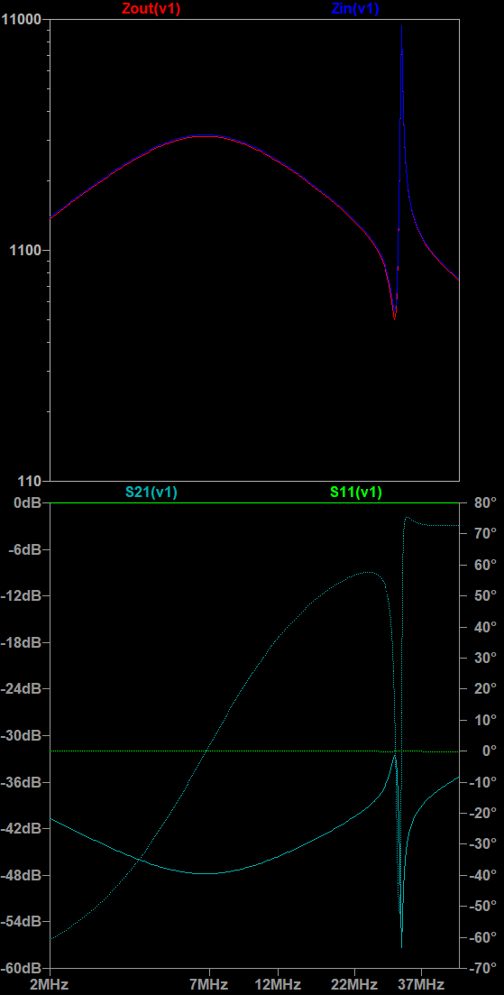 |
Here are inductor impedance (green top curve in each pane)
simulations (just for illustration) of four different models:
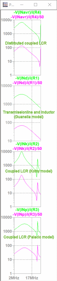
The responce of Guanella equivalent circuit is closest (no spike
around fCO2) to the measurements of the above 1:1
Guanella choke. The reason is that the power-supply chokes are
(multi layer) monofilar inductors, while the MF and HF chokes
(TLT) are a (single layer) bifilar/coax transmission line for
the DM and a inductor for the CM.
Let me know if you have
further improvements.
An equivalent circuit for antenna, Choke and feeder can be found here.
| Ferrite Mix # | Choke | Transformer |
| 31 |
1-300 MHz | 1:1 only, <300 MHz |
| 43 |
25-300 MHz | 3-60 MHz |
| 52 |
200-1000 MHz | 1-60 MHz |
| 61 |
200-1000 MHz | 1-300 MHz |
| 73 |
< 50 MHz | <10 MHz |
| 75/J |
150 KHz – 10 MHz | .1-10 MHz |
.png)
.png)
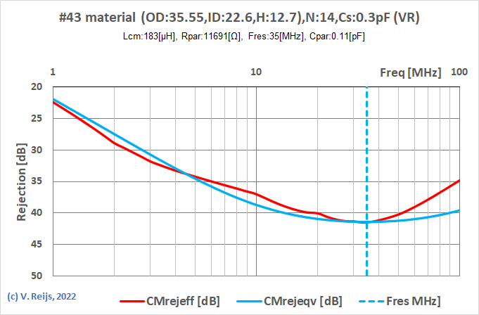
The above model for the Choke is based on variable L(f) and
R(f) and constant Cstray. To simulate this in a
more simplified way (e.g. in LTspice), one could use an
equivalent circuit that approaches the Choke behavior with parallel components
which have fixed values: Lcm, Rpar and Cpar.
The values can be derived from toroid simulation or from a VNA.
Lcm is the inductance at low frequency, aka with μ'i.
Or one can determine it from the low frequency S21
LogMag of a VNA.
Rpar is the highest value of |Zeff|. Or
one can determine it in the S21
|Z|, when the S21 Phase=0
of a VNA. The frequency belonging to this highest |Zeff|
is Fres.
Cpar is now:
Cpar = 1/((2*π*Fres)2*Lcm)
The resulting CMrejeqv (dB, blue curve) below Fres
(dashed blue line) is comparable to the CMrejeff
(dB, red curve) model, but for frequencies above Fres
the simplified model has too much CMR.
| Name |
R0wire [Ω]g | Type |
R0in [Ω] | R0out [Ω] | R0opt [Ω]h | Source |
Configuration |
Picture |
| 1:1 DG0SA (is of the 1:1 Guanella type) |
50 (100||100) |
Choke |
50 |
50 |
50 |
DG0SA https://www.dg0sa.de/341_343.pdf https://www.youtube.com/watch?v=P7wW4TtXmc8&t=2029s |
twice 11 turns bifilar PTFE onto a FT140-43
core. |
 |
| 1:1 Guanella |
50 |
Choke |
50 |
50 |
50 |
DJ0IP https://www.dj0ip.de/vertical-antennas/rf-chokes/1-1-guanella-choke/ |
14 turns RG316 onto a FT140-43 core. |  |
| 4:1 Ruthroff | 100 |
Transformer | 200 |
50 |
100 |
DJ0IP and VK6YSF http://vk6ysf.com/balun_4-1.htm |
16 turns twisted PTFE onto a FT140-61 core.i | 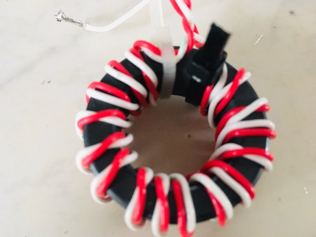 |
| 4:1 Sevick |
100 |
Transformer |
200 |
50 |
100 |
DG0SA https://www.dg0sa.de/341_343.pdf https://www.youtube.com/watch?v=P7wW4TtXmc8&t=2029s https://www.nonstopsystems.com/radio/pdf-ant/antenna-article-trnsmn-lines-2fmi.pdf (page 30-32) |
twice 11 turns bifilar PTFE onto one FT140-43 core. | 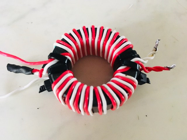 |
| 4:1 dual core Guanella | 100 |
Choke/Transformer |
200 |
50 |
100 |
VK6YSF https://vk6ysf.com/balun_guanella_current_1-4.htm |
11 turns bifilar PTFE onto two FT140-43 core. | 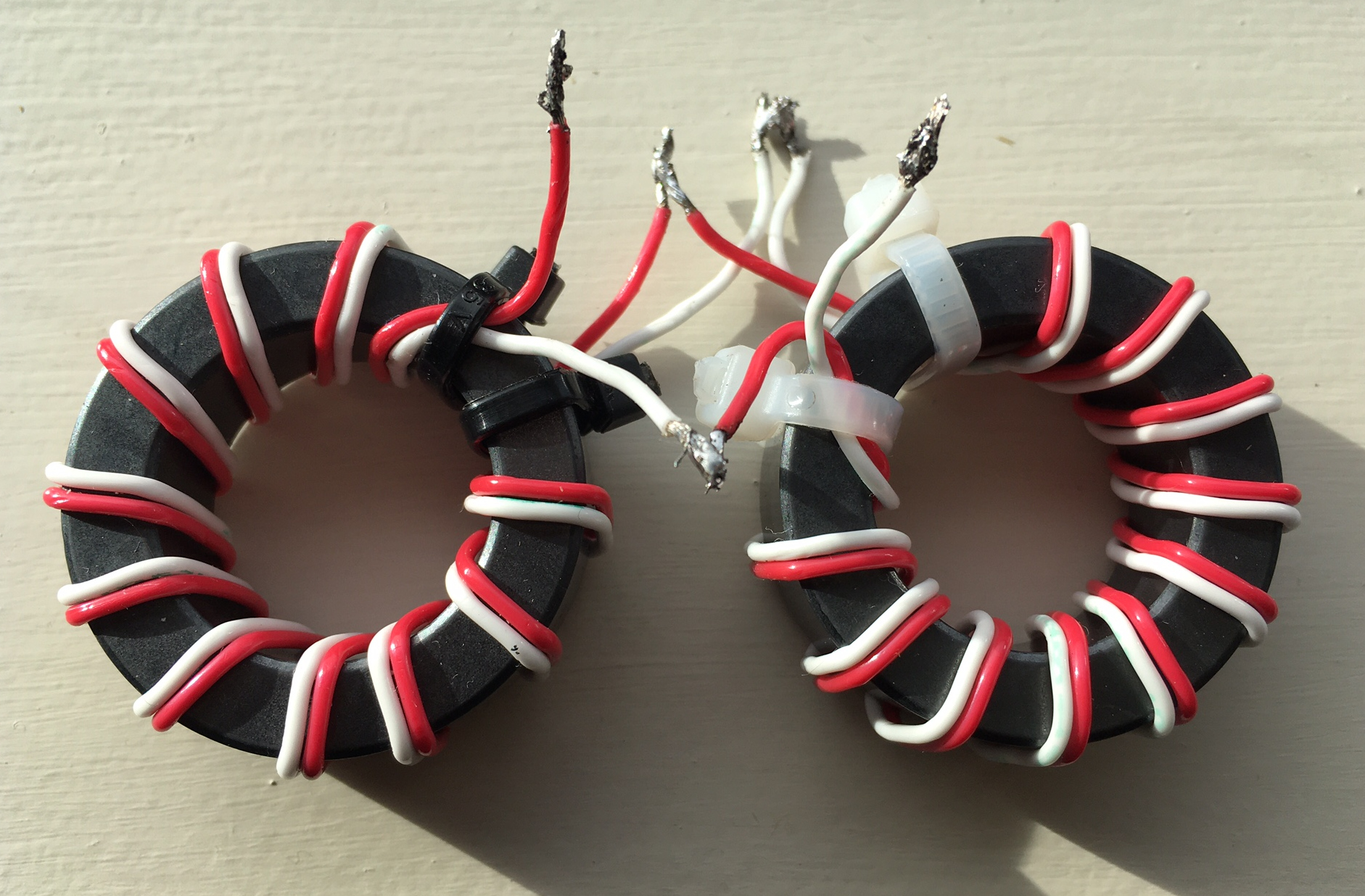 |
The hybrid configuration consists of a Transformer and Choke
defined above.
A picture of a bench-setup for the 4:1 Ruthroff (left) and 1:1
Guanella (right) hybrid configuration (input and output are
terminated with resp. 200Ω and 50Ω; one can conect Earth to the
wiper contact of potmeter, so simulaed resistive antenna):
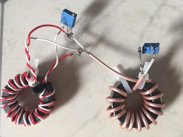
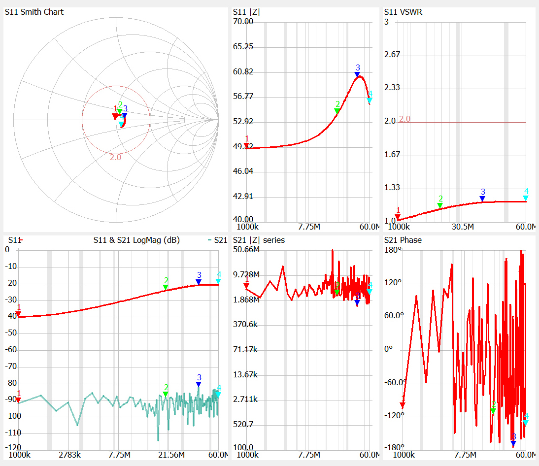
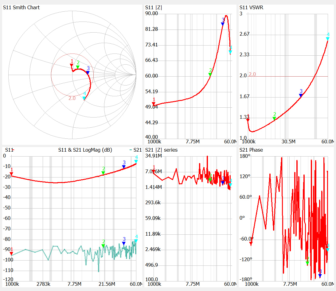
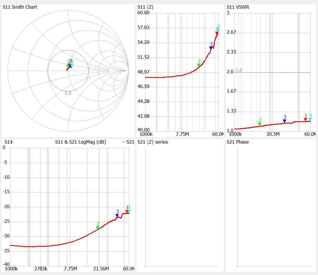
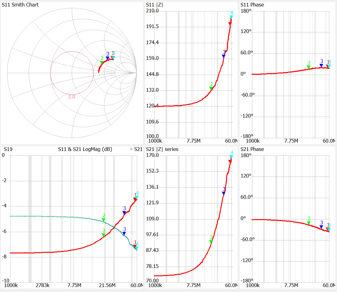
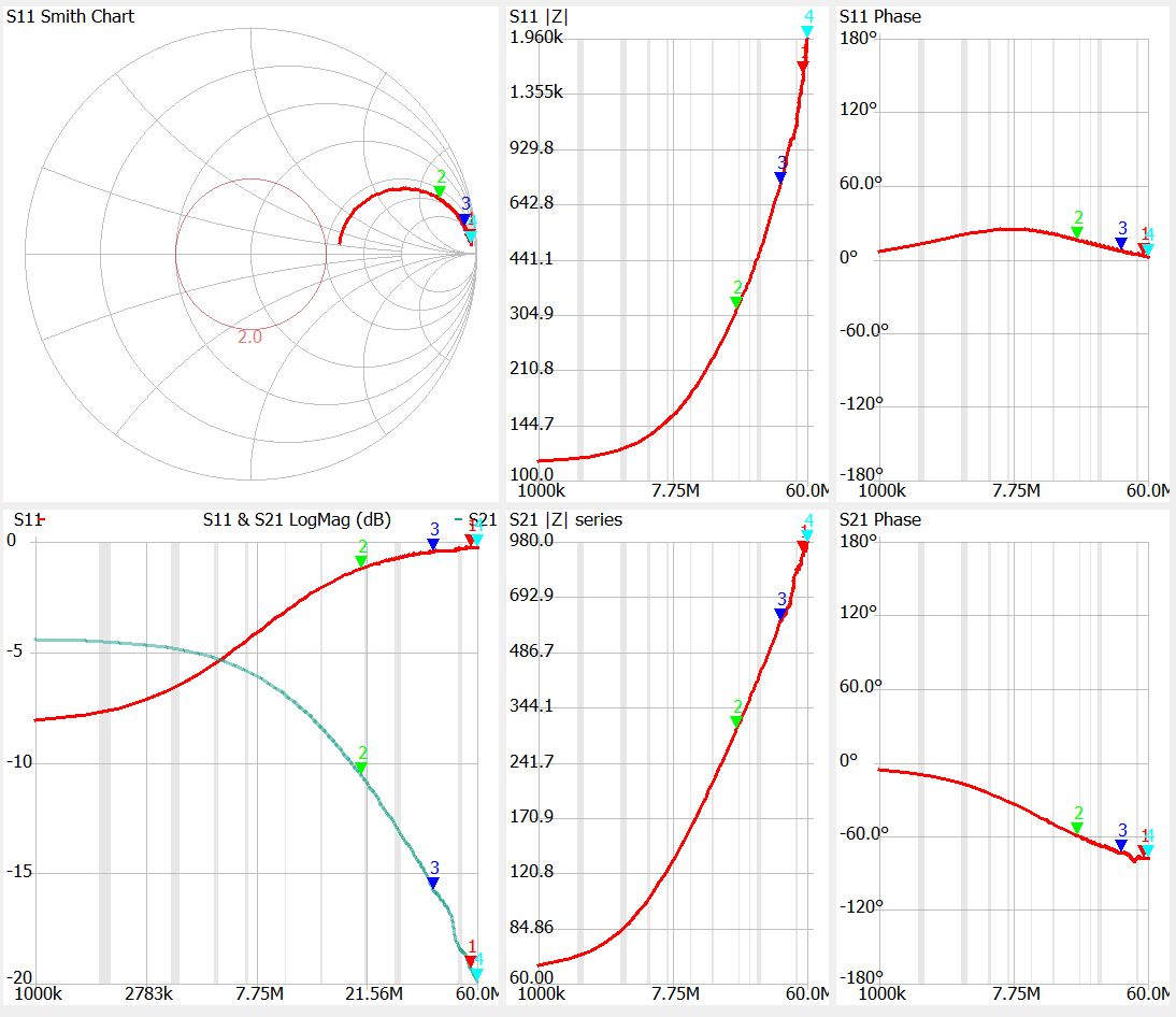
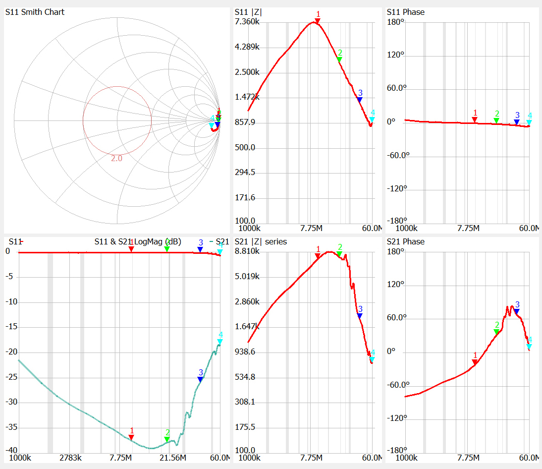
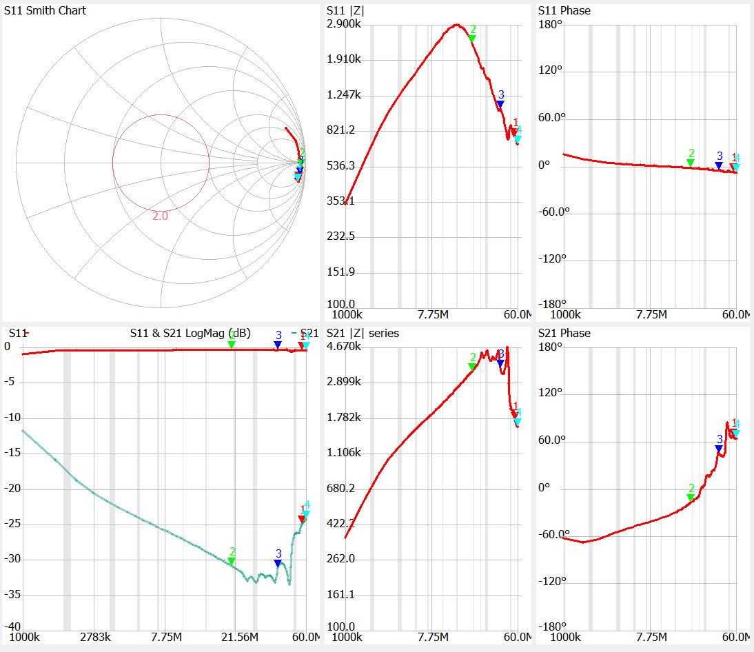
1 port VNA measurements are presented.
For each device the following graphs are shown:
| Transformer
(A) |
Choke (B) |
Hybrid
(A+B) |
 4:1 Ruthroff |
 1:1 Guanella |
 4:1 Ruthroff + 1:1 Guanella |
 4:1 Sevick |
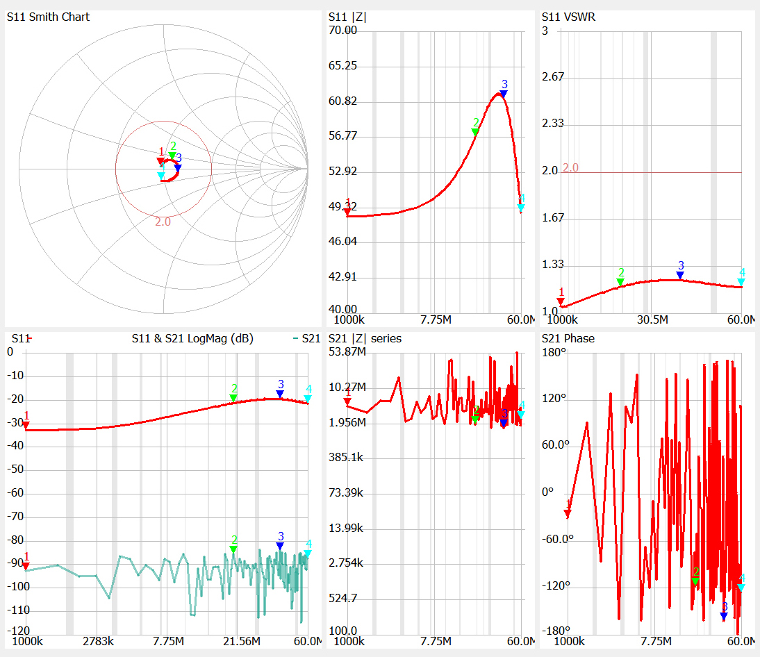 4:1 Sevick + 1:1 Guanella |
|
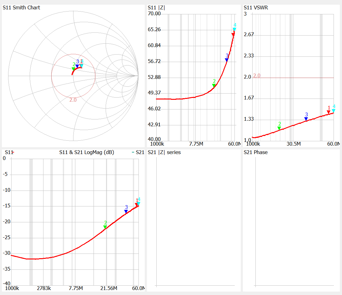 4:1 dual core Guanella |
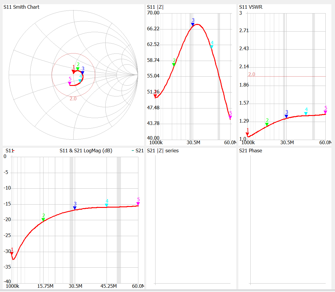 4:1 dual core Guanella + 1:1 Guanella |
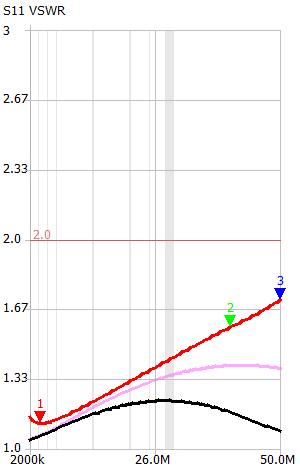
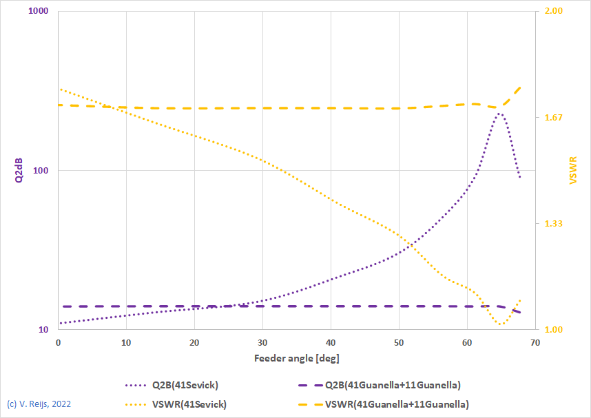
The VSWR can be changed with e.g. a capacitor on 50Ω side of the
Transformer, not on the Hybrid configuration input.
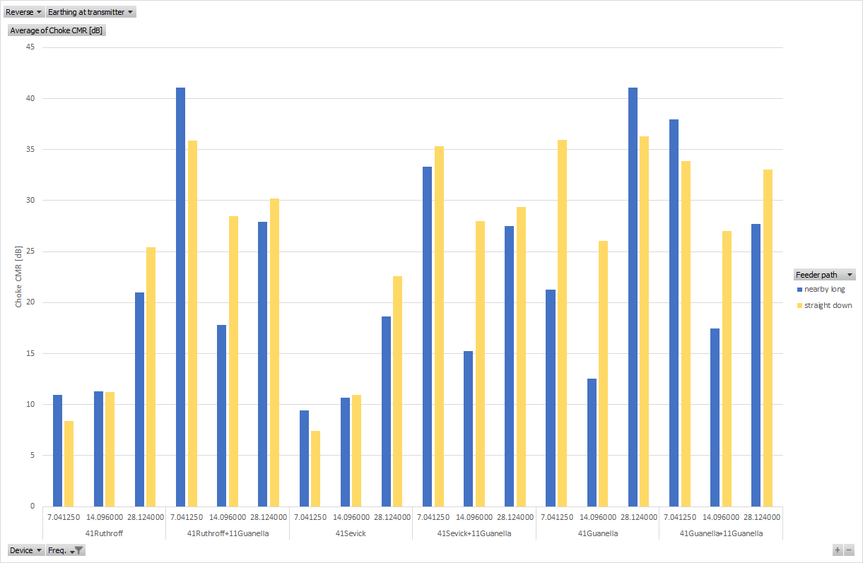
2 port VNA measurements (CM2) are presented.
Below CM2 measurements were done. For each device the following graphs are shown:
| Transformer
(A) |
Choke (B) |
Hybrid
(A+B) |
 4:1 Ruthroff |
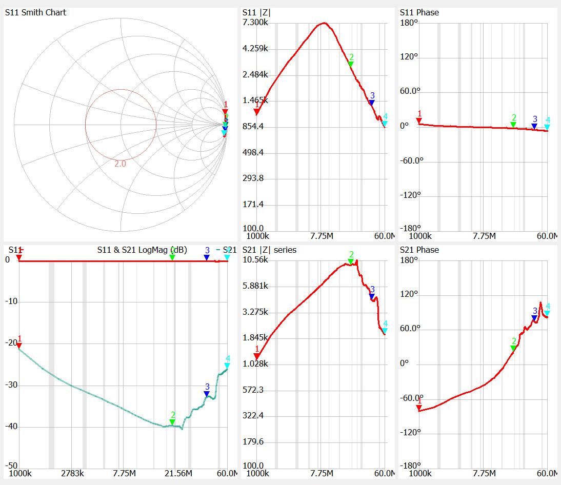 1:1 Guanella |
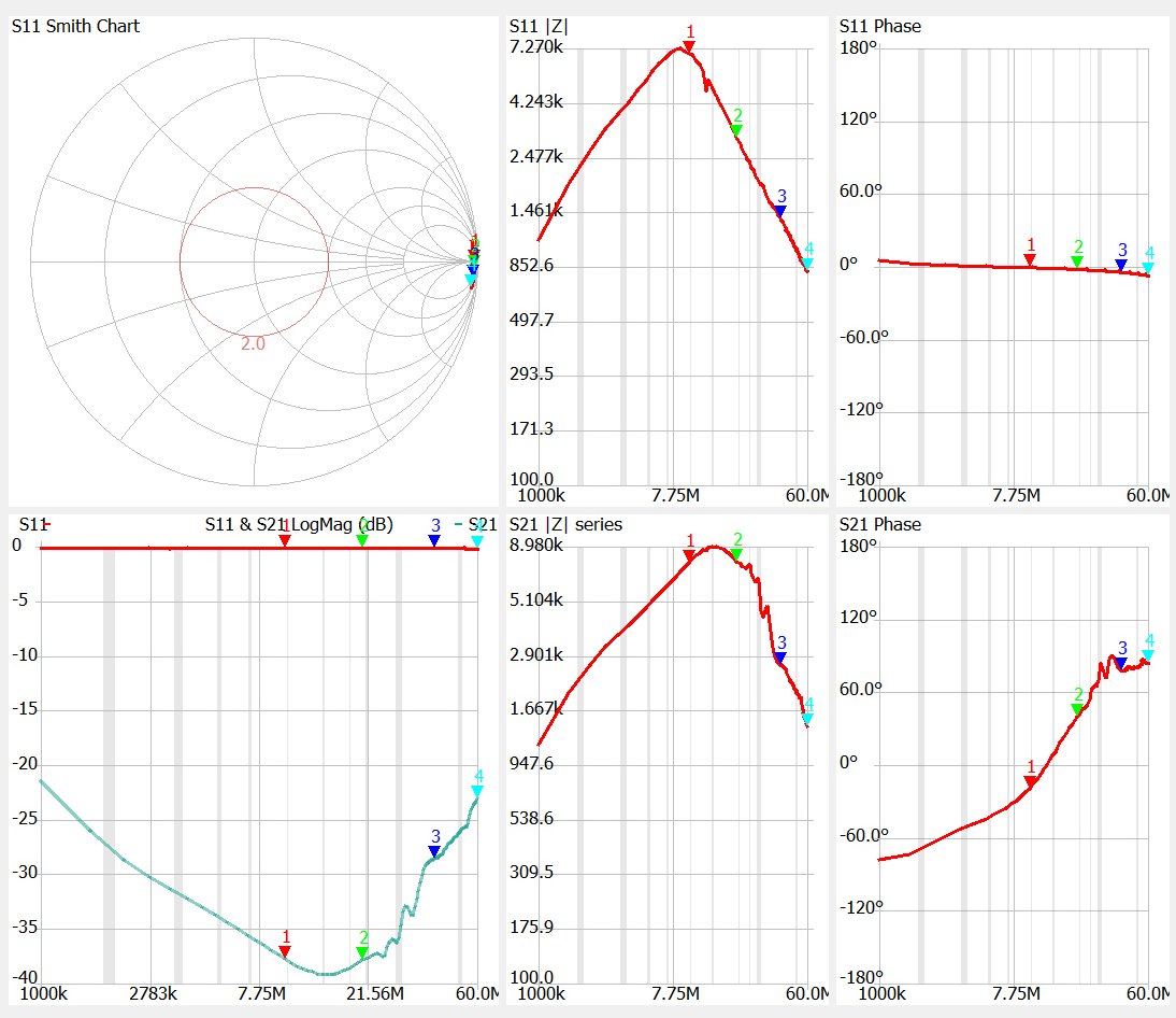 4:1 Ruthroff + 1:1 Guanella |
 4:1 Sevick |
 4:1 Sevick + 1:1 Guanella |
|
 4:1 dual core Guanella |
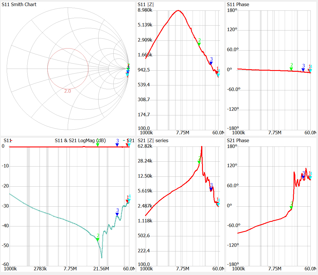 4:1 dual core Guanella + 1:1 Guanella |
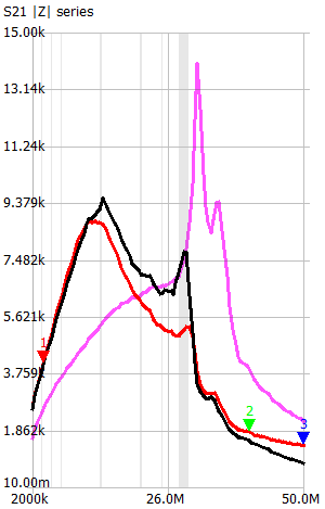
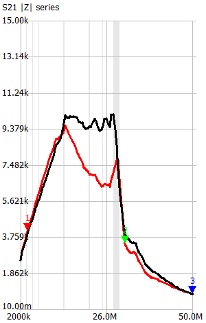
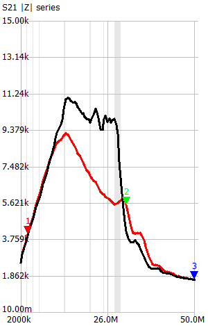
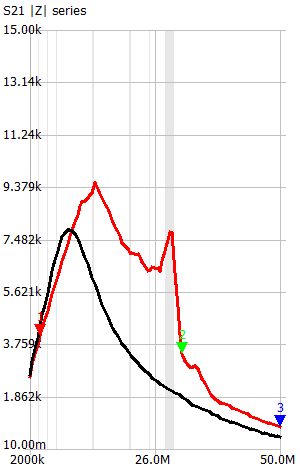
Evaluation of the Hybrid configuration's S21 |Z| series:
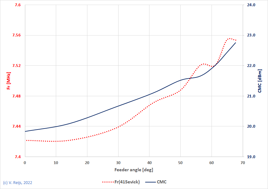
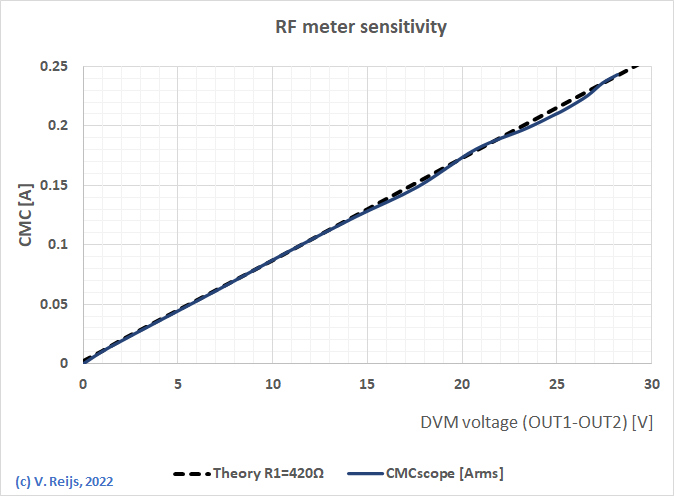
Some other sensitivity test:
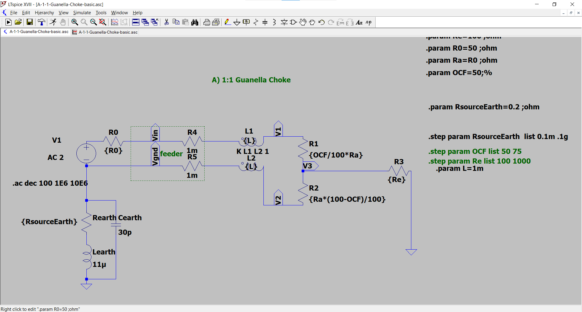
Drawing 5 of G3TXQ needs a slight change to depict reality. The Earth symbol at point c of the coil needs to be removed, and c needs to be connected to b (the coaxial braid). This is reality, as there is normally no Earth available at the location of the Transformer/antenna (if there would be a seperate Earth, Ruthroff Transformer would perform worse looking at CMC).
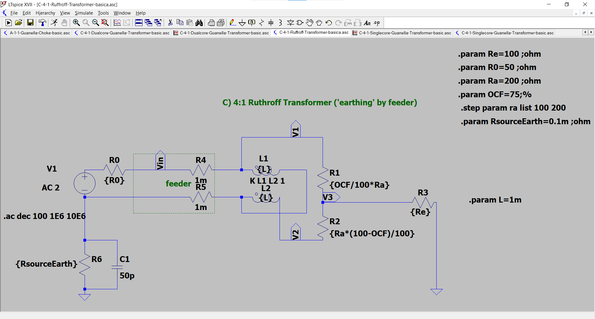
Adjusted drawing 5 of
G3TXQ in LTspice
By a lot of people also called 4:1 single core Guanella
Transformer.
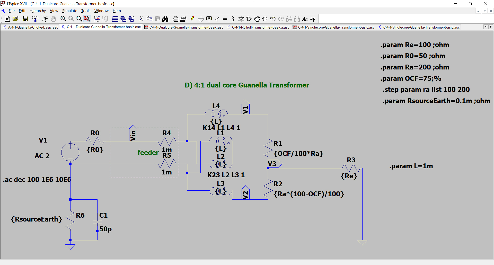
Three parameters are varied: antenna's Earth's impedance
(Re=100 or 1000Ω; which is higher than seen in the Z3
variation of my 40m OCFD measurements),
antenna'a inbalance (OCF=50 or 75%, a balance of 1:3; which is
slightly higher Balance than measured in my 40m OCFD [1:2.4])
and the resistance of source towards Earth (RsourceEarth=1mΩ
or 100MΩ). This gives the below averages in current (ICMC=i(r1)-i(R2)),
voltage (V3) and Rin:
| Type |
Re = {100,1000}
Ω |
OCF = {50,75} % |
RsourceEarth =
{1m,100M} Ω |
||||||
| i(R1)-i(R2)
[A] |
V3
[V] |
Rin
[Ω] |
i(R1)-i(R2) [A] | V3 [V] | Rin [Ω] | i(R1)-i(R2) [A] | V3 [V] | Rin [Ω] | |
| 1:1 Guanella |
7u |
7m |
49.994 |
0.8u |
80u |
50 |
0 |
0 |
50 |
| 4:1 Ruthroff |
75n |
16u |
50.001 |
1.7m |
165m |
48 |
70n |
7u |
50.001 |
| 4:1 Sevick |
1.8m |
400m |
47.7 |
1.7m |
165m |
48.2 |
1.7m |
165m |
48 |
| 4:1 dual core Guanella |
25u |
25m |
49.97 |
4.4u |
440u |
49.996 |
0 |
0 |
50.1 |
| Name |
Type
device |
test 1 |
3.95MHz <freq. too low for the components tested> |
6.9MHz |
14MHz |
comments |
|||||||||
| test
2a
(T) |Z|>???Ω VSWR>150 |
test
3 (T) |Z|~50Ω VSWR<1.2 |
test
4 (C) |Z|~50Ω VSWR<1.2 |
test
5 (C) |Z|~50Ω VSWR<1.2 |
test
2a |Z|>???Ω VSWR>150 |
test
3 |Z|~50Ω VSWR<1.2 |
test
4 |Z|~50Ω VSWR<1.2 |
test
5 |Z|~50Ω VSWR<1.2 |
test
2a ||Z|>???Ω VSWR>150 |
test
3 |Z|~50Ω VSWR<1.2 |
test
4 |Z|~50Ω VSWR<1.2 |
test
5 |Z|~50Ω VSWR<1.2 |
||||
| 1:1 Guanella |
current |
oke |
744/inf |
47.6/1.06 |
47.6/1.06 |
47.3/1.08 |
424/inf |
48.1/1.08 |
48.1/1.08 |
47.8/1.09 |
206/inf |
49.9/1.12 |
49.9/1.12 |
49.6/1.12 |
Test applicable according W8JI, not according Owen
Duffy (not a 4:1 current). Test results are good for a Choke. |
| 4:1 Ruthroff | voltage |
oke |
1.8k/175 |
48.0/1.06 |
2.5/1278 |
13.5/30.0 |
819/168 |
48.0/1.08 |
4.3/137 |
23.2/13.9 |
372/161 |
48.0/1.14 |
8.6/44.9 |
45.9/5.98 |
Test applicable according W8JI, not according Owen
Duffy (not a 4:1 current). Test results are bad for a Choke. |
| 4:1 Sevick | current? |
oke |
892/353 |
48.3/1.05 |
49.9/1.3 |
21.2/7.6 |
486/344 |
48.5/1.05 |
51.3/1.19 |
32.8/3.7 |
232/433 |
49.4/1.08 |
52.3/1.13 |
48.0/2.05 |
Test applicable. Test results are bad for a Choke. |
| 4:1 dual core Guanella |
current |
oke |
1.3k/178 |
48.2/1.06 |
45.9/1.17 |
48.1/1.07 |
826/181 |
48.4/1.08 |
46.6/1.16 |
48.4/1.09 |
307/177 |
49.7/1.15 |
48.1/1.19 |
49.6/1.14 |
Test applicable. Test results are good for a Choke. |
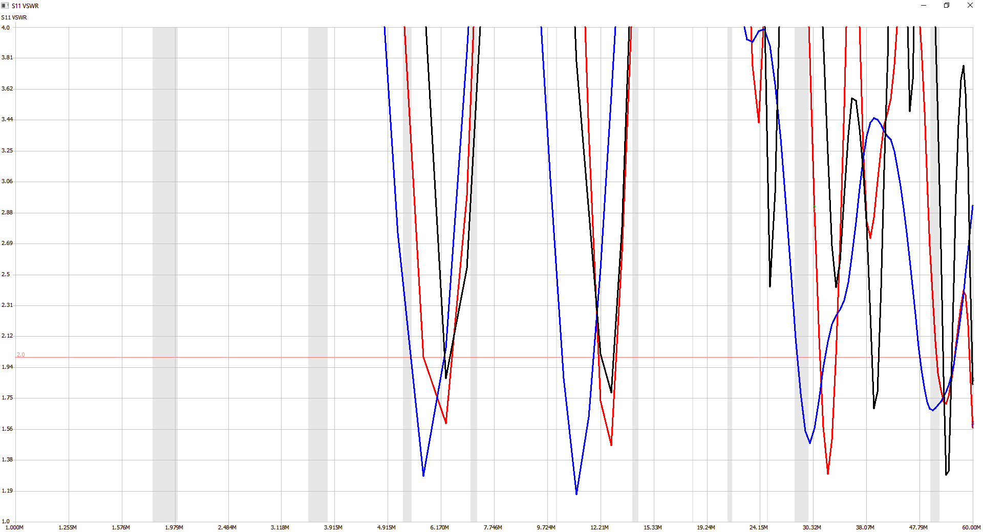
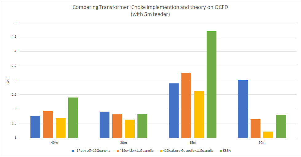
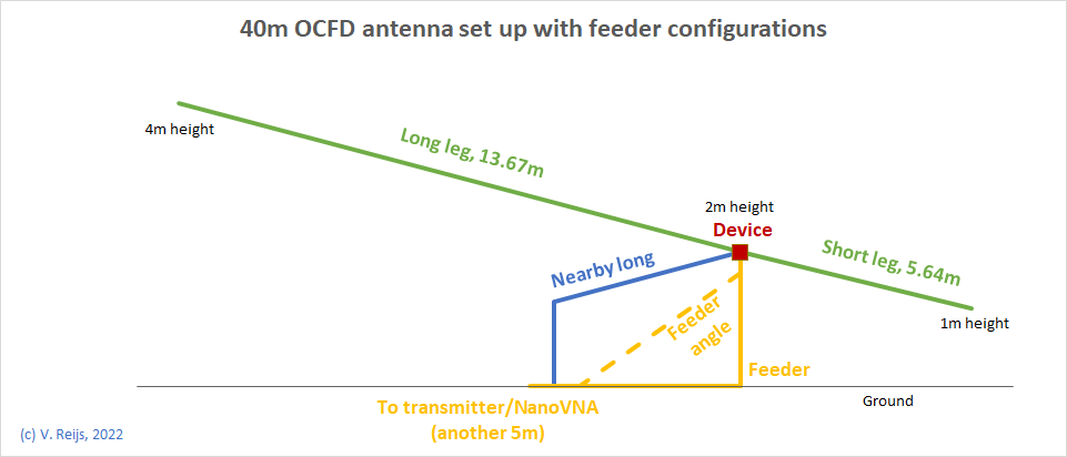
| Band |
measuredd VSWRmin by PE1ATN height=5m ~5m feeder |
measuredd VSWRmin by PE1ATN height=5m ~13m feeder |
measuredd VSWRmin by PE1ATN height=5m ~13m feeder outsidestage |
calculatedb VSWRmin by K8BA height=6m |
||||
| 40m |
1.77@7.1M |
1.92@7.2M |
1.68@7.1M |
1.82@7.2M |
1.73@7.2M |
1.86@7.1M |
1.75@7.1M |
2.40@7.1M |
| 20m |
1.91@13.9M |
1.82@14.5M |
1.64@14.3M |
1.96@14.4M |
1.87@14.4M |
1.78@14.3M |
1.85@14.3M |
1.84@14.0M |
| 15m |
2.89@21.4M |
3.25@21.3M |
2.62@21.4M |
3.59@21.3M |
3.43@21.7M |
2.56@21.4M |
3.73@21.3M |
4.69@21.1M |
| 10m |
3.00@28.3M |
1.65@28.7M |
1.22@28.8M |
1.58@28.7M |
1.57@29.0M |
1.43@28.9M |
1.13@28.9M |
1.80@28.2M |
| xxx-Transformer
+ Guanella Choke (nth repeat measurement) |
RFcable [V] at
different locations on RG-58C/U feeder from receiver |
||
| ~0.5m |
~5.8m |
~11.5m |
|
| 4:1 Ruffroth (1st) | 0.5 |
0.6 |
0.8 |
| 4:1 Ruffroth (2nd) | 0.5 |
0.3 |
0.7 |
| 4:1 Ruffroth (2nd) (device reversed) |
0.7 |
0.4 |
0.6 |
| 4:1 Sevick (1st) | 0.7 |
0.6 |
0.7 |
| 4:1 Sevick (2nd) | 0.7 |
0.2 |
0.4 |
| 4:1 Sevick (2nd) (device reversed) |
0.4 |
0.3 |
0.7 |
| 4:1 dual core Guanella (1st) |
0.8 |
0.5 |
0.5 |
| 4:1 dual core Guanella (2nd) | 1.2 |
1.0 |
0.5 |
| 4:1 dual core Guanella (2nd) (device reversed) |
0.8 |
0.5 |
0.8 |
| 4:1 dual core Guanella (3rd) | 1.0 |
0.8 |
0.5 |
| 4:1 dual core Guanella (3rd) (device reversed) |
0.9 |
0.6 |
0.5 |
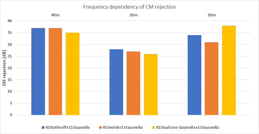
| Freq. [MHz] | RFout [V] | RFcableavg
[V] |
CMR
(field) [dB]* |
CMR (VNA) [dB] |
| 7.0 |
35.5 |
0.5 |
37 |
36 |
| 14.1 |
31.8 |
1.2 |
28 |
37 |
| 28.1 |
24.5 |
0.5 |
34 |
35 |
| Freq. [MHz] | RFout [V] | RFcableavg [V] |
CMR
(field) [dB]* |
CMR (VNA) [dB] |
| 7.0 |
31.8 |
0.4 |
37 |
36 |
| 14.1 |
29.4 |
1.3 |
27 |
37 |
| 28.1 |
20.9 |
0.6 |
31 |
35 |
| Freq. [MHz] |
RFout [V] |
RFcableavg [V] |
CMR
(field) [dB]* |
CMR (VNA) [dB] |
| 7.0 |
38.5 |
0.7 |
35 |
37 |
| 14.1 |
15.5 |
0.8 |
26 |
42 |
| 28.1 | 24.4 |
0.3 |
38 |
41 |
| Type |
40m |
20m |
10m |
||||||
| Freq. [MHz] |
Bandwith
(2dB) [MHz] |
Q2dB |
Freq. [MHz] |
Bandwith
(2dB) [MHz] |
Q2dB |
Feq. [MHz] |
Bandwith
(2dB) [MHz]* |
Q2dB |
|
| 4:1 Ruffroth + 1:1 Guanella |
6.98 |
0.57 |
12.2 |
14.17 |
1.14 |
12.4 |
28.54 |
2.48 |
11.5 |
| 4:1 Sevick + 1:1 Guanella | 7.01 |
0.51 |
13.7 |
14.20 |
1.11 |
12.8 |
28.50 |
2.52 |
11.3 |
| 4:1 dual core Guanella + 1:1 Guanella | 6.98 |
0.49 |
14.1 |
14.14 |
1.14 |
12.4 |
28.46 |
1.84 |
15.5 |
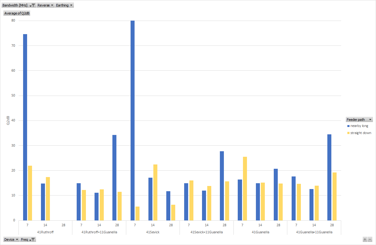
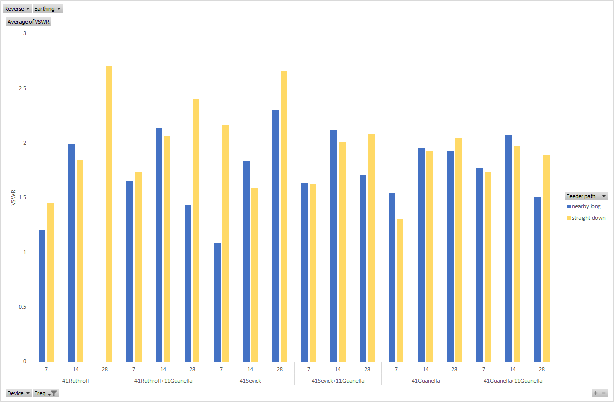
Different feeder path:
Bold purple and underlined text needs
to be studied more. If you can help solve these outstanding
questions, let me
know. Thanks
Outstanding questions: